Simulated Flow Velocity Structure in Meandering Channels: Stratification and Inertia Effects Caused by Suspended Sediment


1
State Key Laboratory of Hydroscience and Engineering, Tsinghua University, Beijing 100084, China
2
Department of Civil and Structural Engineering, University of Sheffield, Sheffield S1 3JD, UK
*
Author to whom correspondence should be addressed.
Water 2019, 11(6), 1254; https://doi.org/10.3390/w11061254
Submission received: 28 April 2019
/
Revised: 9 June 2019
/
Accepted: 11 June 2019
/
Published: 15 June 2019
(This article belongs to the Special Issue Advances in Modelling and Prediction on the Impact of Human Activities and Extreme Events on Environments)
Abstract
:In this study, the coupled effects of sediment inertia and stratification on the pattern of secondary currents in bend-flows are evaluated using a 3D numerical model. The sediment inertia effect, as well as the stratification effect induced by the non-uniform distribution of suspended sediment, is accounted for by adopting the hydrodynamic equations without the Boussinesq approximation. The 3D model is validated by existing laboratory experimental results. Simulation results of a simplified meandering channel indicate that sediment stratification effect enhances the intensity of secondary flow via reducing eddy viscosity, while sediment inertia effect suppresses it. The integrated effects result in an increase and a reduction in the secondary flow, respectively, at lower and higher concentrations (near-bed volumetric concentrations of 0.015 and 0.1 are, respectively, considered in this study). This suggests that the dominance of the suspended sediment effect depends on the sediment concentration profile. With the increase of concentration under a specific sediment size, the secondary flow rises to reach a maximum, and then decreases. Moreover, as the sediment concentration increases, an exponentially decaying rate has been found for the secondary flow. It is concluded that in the numerical simulation of flow in meandering channels, when concentration is high, the variable-density hydrodynamic equations without the Boussinesq approximation should be considered.
1. Introduction
In fluvial process studies, suspension has always been known to have a fundamental role in defining the preferential bend migration, since the stratification brought by suspended load modifies the turbulence, flow structure and sediment entrainment. Early works relate sediment stratification effect on flow velocity to concentration profiles. Vanoni [1] and Einsterin and Chien [2] classically documented the sediment stratification effect on the velocity profile in turbulent open channel flows. Vanoni showed that the von Karman constant κ reduces at high sediment concentration. This was based on the hypothesis that the suspended sediment dampens turbulence and increases velocity gradient near the wall. Later, many laboratory investigations [3,4,5] confirmed this finding. Castro-Orgaz et al. [6] analytically indicated that the reduction of κ in the high concentration condition is a physically coherent approximation. Suspension stratification effect modulates the turbulence intensity which in turn reduces the vertical sediment diffusivity. A few attempts referred the suspension effect to heat or salinity induced stratification effect [7]. By analogy with thermally stratified boundary layers, the Flux Richardson number or the gradient Richardson number for sediment-laden flow is defined as a measure of stratification effect or turbulence damping [8,9] and the Monin-Obukhov length scale is introduced to establish damping functions for the eddy viscosity [10]. Herrmann and Madsen [11] obtained the optimal parameters for damping eddy diffusivity from observations. Nezu and Azuma [12] presented simultaneous measurements of both sediment and fluid in dilute flows. They pointed out that flow turbulence intensity is slightly dampened far from the bed while it rises in the near-wall region owing to the velocity difference between fluid and sediment. The ratio of concentration to slope is a primary indicator of stratification effect (which is greater in low slope rivers) according to Wright and Parker [13]. For high suspension concentration, Lamb et al. [9] experimentally observed that the Richardson number critical value of ~1/4 for completely damped turbulence [7] is not applicable where the major source of suspension is transported turbulence; and Muste et al. [14] provided the priority of two-phase over traditional mixed-flow perspective on sediment laden flows from image velocimetry experiments.
Although sediment laden flows have been widely studied by using various numerical models, most studies concern low suspension concentration using the advection-diffusion equation. The fundamental assumptions of these models limit their applicability. The advection-diffusion theory regulates the upward transfer of suspension due to turbulent diffusion with the downward settlement. Winterverp [15,16] numerically explained the sediment stratification effect by a buoyancy destruction term in the standard k-ε turbulence model at low concentration. Later, concerning hindered settling, van Maren et al. [17] extended this explanation to hyperconcentrated flows. Byun and Wang [18] coupled the sediment transport model and the 3D tidal hydrodynamics model to examine the reduction of turbulence and bottom shear stress due to the sediment stratification effect. Amoudry and Souza [19] performed 3D simulations and showed that sediment stratification effect leads to non-negligible modifications for bed evolution. Cantero et al. [20] exploited Direct Numerical Simulation (DNS)s of sediment laden flows under the dilute flow assumption and Boussinesq approximation. For higher settling velocity, the vertical Reynolds fluxes could be completely suppressed locally and relaminarization occurs [20,21]. For the condition of complete turbulence suppression, the critical product of the Richardson number and sediment settling velocity has a logarithmic dependence on the Reynolds number [22]. Dutta et al. [23] further investigated the sediment stratification effect on the vertical sediment diffusivity by DNSs. Dallali and Armenio [24] used Large Eddy Simulation (LES) to investigate suspension transport, supporting that the buoyancy effect on flow momentum is not neglectable for small particles. Alternatively, two-phase flow theory addresses water and sediment phases separately [25]. Recently, several models based the two-phase flow theory have been developed to include small scale mechanics [26,27,28]. The drift velocity shows that the inertia of fluid, particle turbulence and collisions effect contribute to sediment dispersion [26].
The Boussinesq approximation [29] is the basis for mathematical formulation of various flow problems. According to Kundu and Cohen [30], after subtracting a static reference state, i.e., (, where ρ0 and p0 = reference mixture density and pressure, and = acceleration of gravity), the momentum equation can be expressed as
where t = time; p′ and ρ′ = local deviations of pressure and mixture density from static reference state; = flow velocity vector; and ν = kinematic viscosity.
Both the inertia and buoyancy terms (the term on the left-hand side and the second term on the right-hand side of the above equation, respectively) contain the density ratio. With the Boussinesq approximation, the sediment stratification effect is shown as the buoyancy term while the inertia effect (the density ratio in the inertia term) is neglected. One then has
Sediment concentration near the water surface is always much lower than that near the bed for the condition of heavy particles. A large vertical density gradient which has obvious inertia effect on flow can be a result of high bulk sediment concentration. The vertical concentration gradient is often very large with significant inertia variations. Therefore, the applicability of the Boussinesq approximation needs to be assessed in such a case. To the best of our knowledge, there have been no reported documents on the numerical comparison of sediment laden open-channel flows with and without considering the Boussinesq approximation.
Because the role of fluid inertia is highly important in the acceleration/deceleration processes of fluid flow, a 3D modelling method is adopted to thoroughly analyze the inertia effects of suspended sediment under complicated flow boundary conditions. The 3D model is substantially different from traditional hydrodynamic models under Boussinesq approximation which only consider the stratification effect of suspensions as the buoyance term. In the following sections, first, model setup is provided; second, a few cases are selected for model verification; third, numerical experiments with and without Boussinesq approximation are presented for comparison; and finally, discussions and suggestions with regards to the sediment inertia effect are given.
2. Model Setup
2.1. Hydrodynamic Model
The governing hydrodynamic equations are 3D shallow water equations based on the hydrostatic pressure. The mass and momentum equations are written as follows:
where x, y and z = Cartesian coordinates; u, v and w = components of velocity in the x, y and z directions; p = pressure; ρ = density of mixture; and νh and νz = eddy viscosity in the horizontal (x and y) and vertical (z) directions. The density of the mixture is determined by
where c = volumetric concentration of sediment; ρw = water density; and ρs = sediment density.
Similar to layer-integrated models [31,32], the vertical velocity is calculated from the integrated continuity equation as follows
where zb = bed elevation; and wzb is the vertical velocity at the bed. At the water surface,
where H = water surface elevation.
The pressure in the horizontal momentum equations is given by integration of vertical momentum equation as
where pa = pressure at the water surface which is set to zero in the present simulations. The pressure gradient is obtained as follows
Eddy diffusivity and viscosity are obtained from a two-equation k-ω turbulence closure model [33]. Complete extinction of local turbulence is unsustainable according to Cantero et al. [22]. To prevent the turbulence to be totally damped by the sediment stratification effect, a prescribed upper threshold 0.2 is set on the flux Richardson number. As the Reynolds-Averaged Navier–Stokes (RANS) model is incapable of modeling flow under conditions of strong stratification [34], an empirical distribution [25] for viscosity is reserved here as follows.
where h = water depth; and U* = friction velocity.
2.2. Sediment Transport Model
Sediment transport is represented by the advection-diffusion equation,
where wf = sediment settling velocity; and εh and εz = eddy diffusivity in the horizontal (x and y) and vertical (z) directions.
2.3. Boundary Condition
There are two thin layers of δ at the water surface and the bed boundaries, thus the thickness of the calculation domain is h − 2δ. Vertical boundary conditions are implemented at these two interfaces. Normal gradients of horizontal velocities as well as the net vertical flux of sediment are zero at the upper interface. At the bottom one, we enforce the bottom frictional stress for momentum equations as
where ub and vb = near-bed components of horizontal velocity; and CD = drag coefficient to be calibrated. Besides, the near-bed net flux of sediment is
where qsu = sediment entrainment rate; and cb = near-bed volumetric concentration.
Flow condition at the inlet is given by flow discharge. In other words, the flow velocity profile at the inlet can be estimated through the transport equation for turbulent components and momentum equations with the assumption that flow is locally uniform at this boundary. Similarly, the suspended sediment concentration profile at the inlet is determined by assuming local equilibrium in the inlet sediment entrainment. At the outlet, the water level is set to prescribed values as the flow is assumed to be subcritical.
2.4. Domain Discretization
For discretization of the computational domain, a Spectral Element Method (SEM) is used in the vertical direction (due to the importance of the vertical variations in the present work) and the finite difference method is employed in the horizontal directions. Besides, for ease of implementation of the boundary conditions, vertical domain is discretized into three layers (due to the existence of two thin layers adjacent to water surface and bed) with unstretched z-coordinates. First, vertical space is divided into a number of sublayers with evenly thickness of h0. The top/bottom sublayer is combined with its adjacent sublayer, producing a layer with a thickness between h0 and 2h0. Then, all the rest inner sublayers are combined to form an inner layer with its thickness being multiple of h0. Therefore, there will be three vertical layers throughout the whole calculation domain. All these three layers are variable according to water surface and bed changes during calculation process. Thickness thresholds zmin and zmax are imposed over top and bottom layers. When the thickness of the top/bottom layer is out of range (>zmax or <zmin), after the calculation of water surface/bed elevation at a certain time step, the layer interface will move a distance of h0 inward or outward to ensure the thickness stays in the range. Let h0 = (zmax − zmin)/2, after adjustment, its thickness will be close to (zmax − zmin)/2. Then, there is no need to readjust the thickness for small surface/bed changes. Every thickness adjustment is accompanied by local redistribution of physical quantities.
This kind of vertical discretization allows us to conveniently employ the finite dimensional space/polynomial of relatively higher degree for inner layer and lower degree for top/bottom layers. For the horizontal diffusion/viscosity calculations at the inner layer, if the horizontally adjacent inner layers are consistent, the calculations will be straight-forward as in the z-coordinates method, otherwise, additional interpolations need to be carried out separately for each calculation. For the calculations at the top/bottom layer, the horizontally adjacent layers are always inconsistent, and interpolations are required.
Horizontal domain is discretized using curvilinear coordinates into staggered grids. The governing equations need to be converted accordingly for implementation. Here, we present only the framework in the Cartesian coordinates for simplicity.
2.5. Solution of Generalized Equation by SEM
The horizontal momentum, sediment and turbulence transport equations can be generalized as
where ϕ = the physical quantity to be solved; wf is set only for sediment transport; σ = the Prandtl–Schmidt number for ϕ; and f = other terms. The top and bottom boundaries are chosen according to the specific equation to be solved. At each vertical layer i with thickness Li = zi+1 − zi, generalized equation is conducted under local vertical coordinate ζ = 2 (z − zi)/Li − 1. We set an approximation such that ϕ belongs to the finite dimensional space of degree N. Choosing the Legendre polynomials as the local basis functions, the approximate solution is defined by
where ϕk and hk(ζ) = the coefficients and the Lagrange form of Legendre polynomials, respectively; interpolation point ζk = Legendre–Gauss–Lobatto point with its weight ωk; and and = the Legendre polynomials and their derivatives. Generalized equation is multiplied by the test function and integrated over ζ (between [–1, 1]) and time step. We choose the local basis function as the test function. Then, the weak formulation after including boundary condition, can be derived as
The integral coefficients are given as
where = the weighting function of Gaussian quadrature for ζj. The depth integrated continuity and horizontal momentum equations are solved in the coupled way.
Depth integrated continuity equation is discretized with a semi-implicit approach in curvilinear coordinates as
where ξ and η = horizontal curvilinear coordinates; and = depth-averaged values of u and v; θ = the implicitness factor for temporal discretization; and = Jacobi determinant. Substituting the discretized continuity equation into the horizontal momentum equations,
where =; ν = νh for simplification; σ = Schmidt number; and um*n = the backtracked value of um at time step n. Momentum equation for v has a similar form. Underlined terms are zero at the outlet for imposing water level condition for subcritical flows. In the momentum and sediment transport equations, advection terms are incorporated in the total derivatives. By backtracking characteristic lines accurately under Eulerian–Lagrangian context [35], the backtracked value at the foot of the characteristic lines at time step n can be approximated by interpolation. The final set of momentum equations can be solved by Conjugate Gradient. Equation (21) is semi-implicit with respect to v. Hence, v is firstly taken as an explicit quantity in the horizontal momentum for u, and then one more iteration is applied after the solution of the horizontal momentum equations. Once the horizontal velocities are known, water surface level and vertical velocity can be computed using the depth integrated continuity equation.
3. Model Verification and Results
The developed 3D numerical model is employed to simulate flow and suspended sediment transport in straight and meandering channels, and validated by comparing the measured and predicted distributions of flow hydrodynamics and sediment transport characteristics. To examine the effect of suspended sediment on the flow structure, a meandering channel flow with considerable suspended sediment is considered. As there was no experimental data available to us for suspended sediment motion in meandering channels, we firstly validated the model for the cases with suspended sediment at equilibrium and non-equilibrium conditions in straight channels with comparing the model results with a set of existing experimental data (Section 3.1); then applied the model for a meandering channel (but without presence of suspended sediment, i.e., only clear water) and validated the accuracy of the model against existing experiments (Section 3.2); and finally, numerically simulated flow and sediment motion in a meandering channel with investigating the effects of suspended sediment on the velocity structure (Section 3.3).
3.1. Uniform and Steady Open Channel Flows
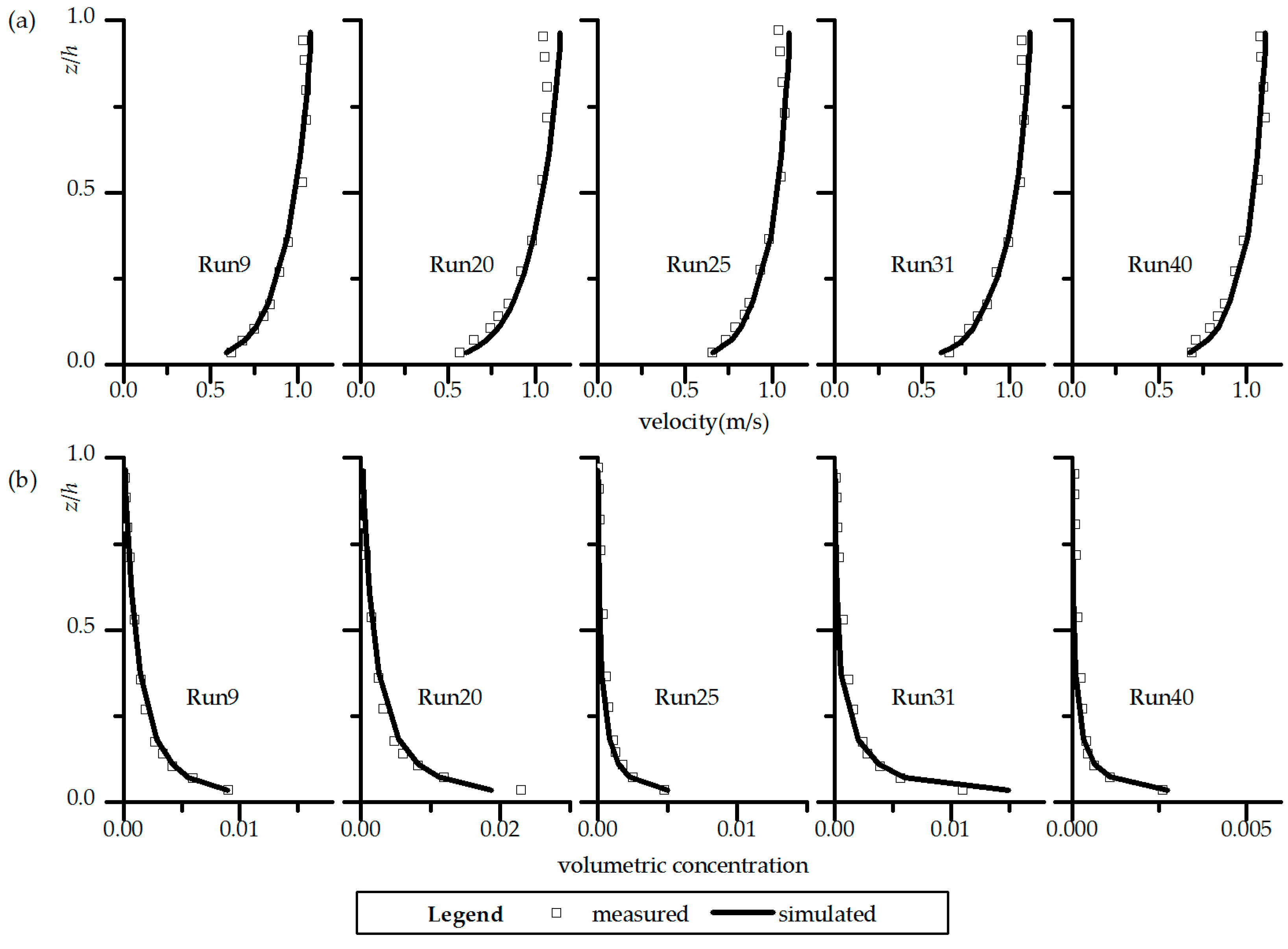
A data set of laboratory experiment carried out by Coleman [36] was used to verify the model for flows with suspended sediment at equilibrium condition. The experiment was carried out in a 15 m long and 0.356 m wide recirculating flume with the slope of ~0.002. The measurements were taken at 12 m downstream of the inlet. The flow discharge and depth were ~0.064 m3/s and ~0.169 m, respectively. The velocity and sediment concentration were measured with a Pitot-static tube. Forty runs were performed with sediments of three different grain diameters and different concentrations. Runs 9, 20, 25, 31, and 40 are selected for comparisons with numerical results. Diameter of the sand grains were about 0.105, 0.210, and 0.420 mm, respectively, in runs {9 and 20}, {25 and 31}, and {40}. The Schmidt number for sediment vertical diffusivity is closely related to sediment diameter. Hence, we use the Schmidt numbers of 0.7, 1.2, and 2, respectively, for those runs.
Figure 1 presents the estimated velocity and sediment concentration profiles in comparison with the experimental ones. A good agreement between them is observed except in the upper part of the profiles, i.e., near the water surface. One reason could be that the effects of lateral walls on the flow are neglected in the present simulations, while those effects could be relatively high in the present case due to the low aspect ratio (width to depth) of the flume.
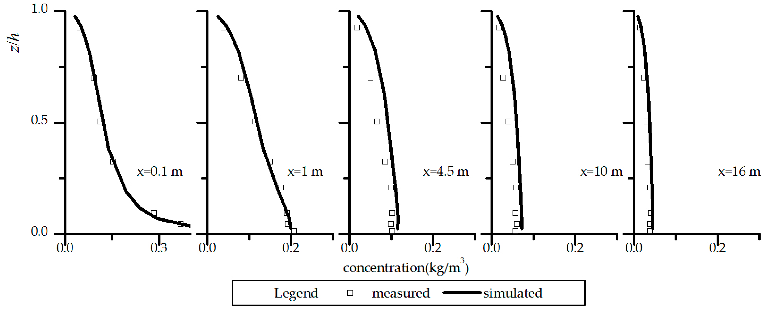
The model performance is tested for non-equilibrium condition, too. The non-equilibrium suspended sediment laboratory experiment of Wang and Ribberink [37] is considered. This experiment was carried out in a 30 m × 0.5 m × 0.5 m straight flume with a slope of 0.00097. The flow was 0.216 m deep and the discharge was 0.0601 m3/s. The flume was composed of a 10 m inflow section with a rigid bed, a 16 m test section with a perforated bed and a 4 m outflow section. Sediment was released at upstream section through the water surface. Nearly uniform sediment was used with settling velocity of wf = 0.007 m/s. The velocity was measured with a micropropellor and the sediment concentration was estimated by using the siphon method. The sediment profile was calculated at the inflow section as in an equilibrium state under given near-bed condition of qsu = 1.19 × 10⁻⁶ m/s. In the test section, qsu was set to zero. According to Wang and Ribberink [37], fluctuations were observed in the measured profile of the sediment concentration.
The numerical result is presented in Figure 2 in comparison with the experimental data. The comparison implies that the model performance is quite good for the non-equilibrium condition, too. The model is thus validated for the flow with suspended sediment at equilibrium and non-equilibrium conditions in straight channels.
3.2. Steady Flows in Meandering Channels
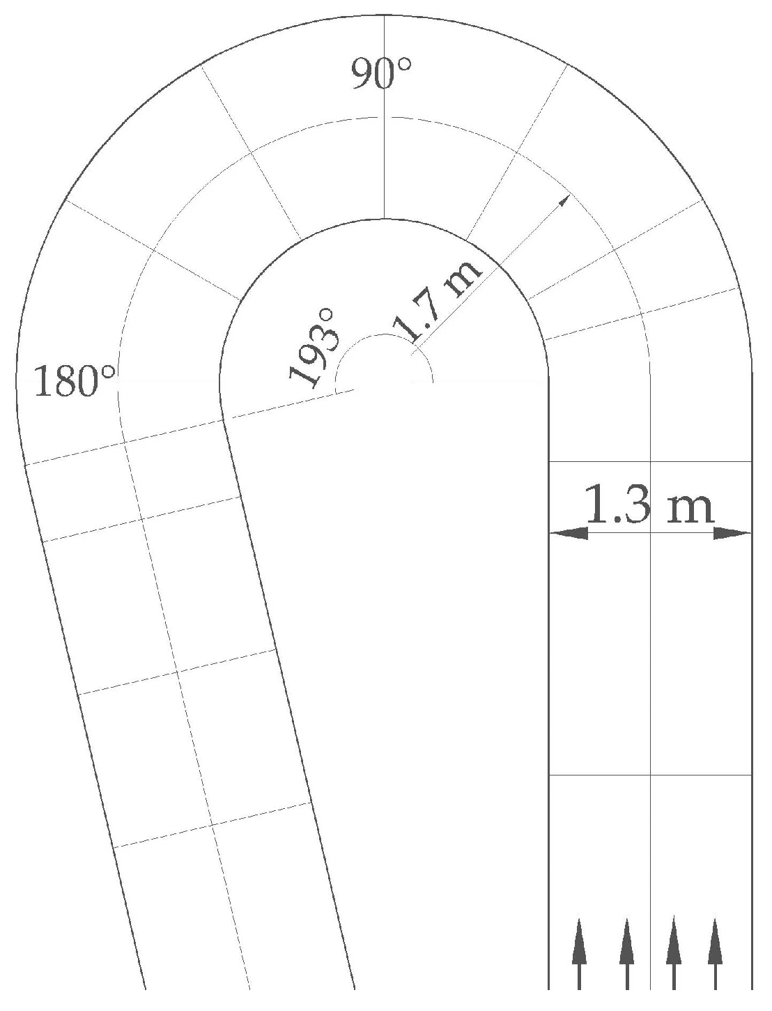
The sharp bend experiment of Blanckaert [38] is used for model evaluation in curved bend flows. The experiment was carried out in a zero-slope flume consisted of a 9 m straight inflow, a 193° curved bend and a 5 m straight outflow section (Figure 3). The curvature radius of the bend was R = 1.7 m. The width of the channel was B = 1.3 m, and the lateral walls were vertical and hydraulically smooth. The velocity was measured by an acoustic Doppler velocity profiler. For the present simulation, we selected one steady case with the water depth of 0.159 m and discharge of 0.089 m3/s.
The calculation was performed on a horizontal staggered grid with 130 × 20 cells. Calculation domain contains the curved bend and two 2.6 m length sections of inlet and outlet. The time step was set to 0.1 s. Inlet depth was identical to the measured one after adjusting the drag coefficient. Friction resistance is not taken into account for the side walls.
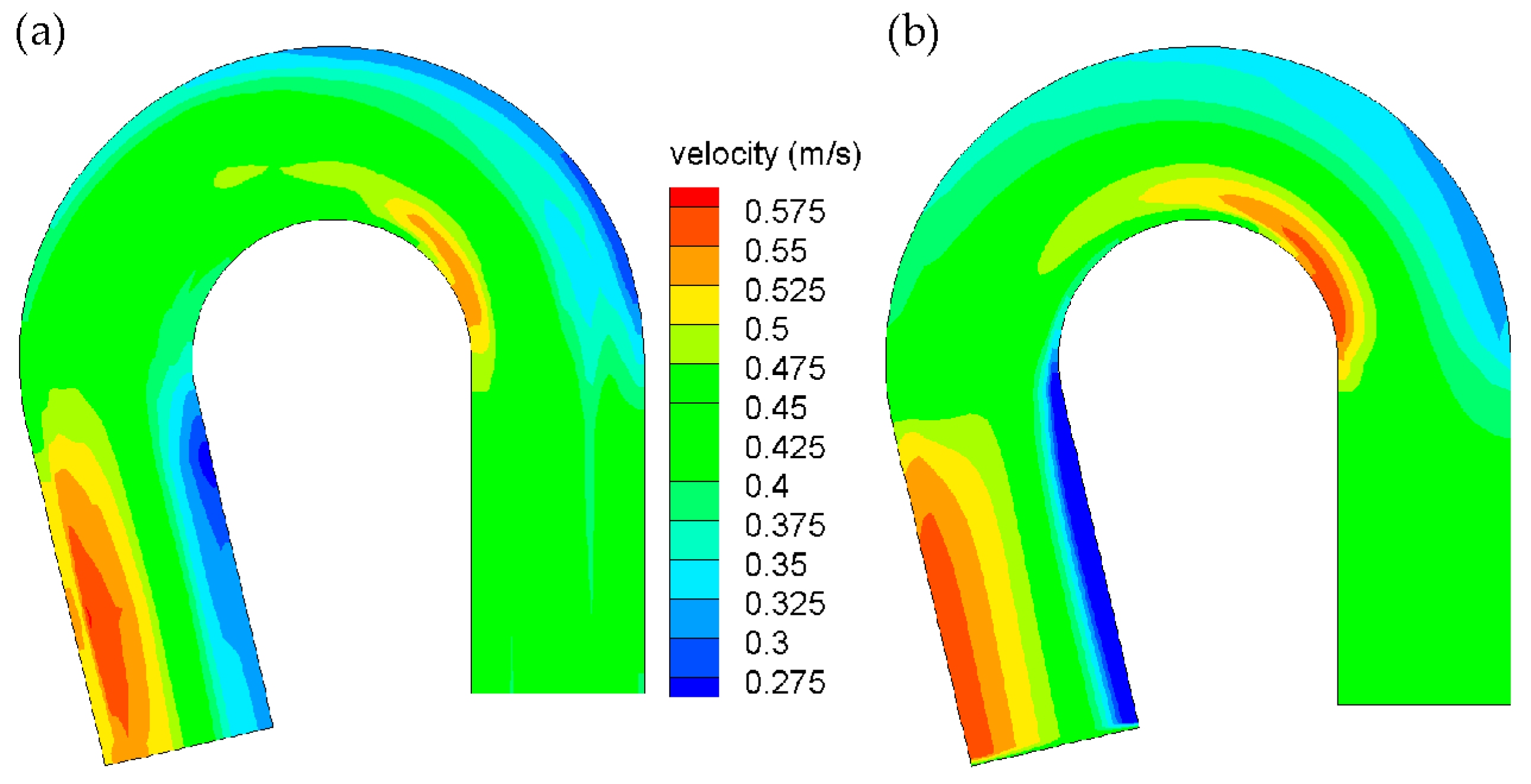
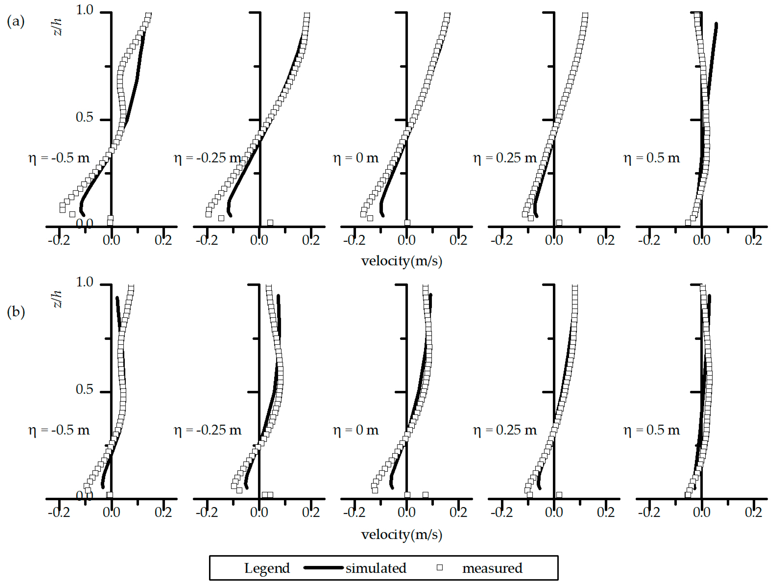
Figure 4a shows the distribution of the measured depth-averaged streamwise velocity. The short flow route leads to an acceleration close to the inner bank which is strengthened by transversal pressure gradient. At the same time, the streamline curvature induced a cross-sectional secondary flow, which shifts the larger velocity core toward the outer bank. These two mechanisms together generate the gradual outward shift of the larger velocity core at the channel bend. In the present calculation, magnitude of vertical viscosity is set to half of the horizontal one. Figure 4b shows the result of the numerical model. Outward shifting process of larger velocity core is closely consistent with the experiment. Figure 5 presents the streamwise velocity profiles in comparison with the experiments at two cross-sections shown on Figure 3, i.e., cross-sections 90° and 180°. Although the present model is hydrostatic with isotropic turbulence model, only some small local differences with the experiment are observed near the side walls (Figure 5). Figure 6 presents the estimated transverse velocity profiles at the same cross-sections in comparison with the experimental data. It shows that the model is also capable of predicting transverse velocity with good accuracy.
3.3. Effects of Suspended Sediment on Velocity Structure
Flows in curved open channels modulate the velocity components both in the streamwise and transverse directions as shown previously. Inertia of flow plays an important role in the acceleration and deceleration processes. In the dilute sediment laden flows, the mixture density can be approximately treated as a homogeneous quantity, thus the effect of sediment inertia can be neglected. Since sediment has a greater density than water, if concentration increases, how the sediment inertia affects the laden flow is still unclear. To investigate this issue, here, we carry out a numerical study on the inertia effect in a meandering channel. Channel geometry and flow discharge in Section 3.2 are adopted. The parameters employed in the simulation are reported in Table 1. The simulations are carried out both with and without considering the Boussinesq approximation, with investigating the effect of near-bed volumetric concentration cb. Runs BAL and N0L are those with and without the Boussinesq approximation for cb of 0.015; and runs BAH and N0H are also with and without applying the Boussinesq approximation but for a higher concentration, i.e., cb of 0.1. Run CL, which is the clear water case presented in Section 3.2, is also included for comparison.
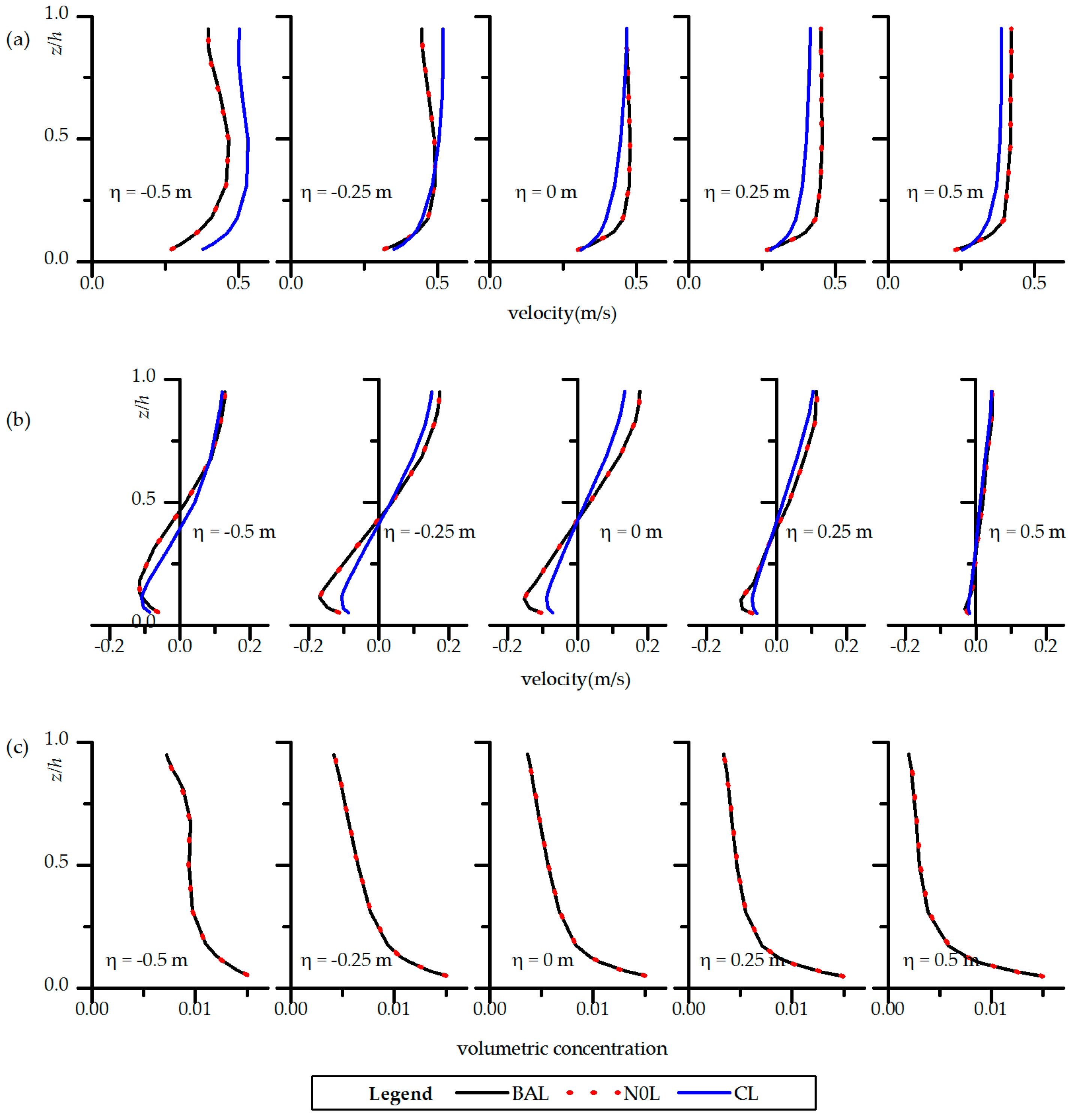
According to the results of the simulations, all the runs have similar water surface elevation distributions with different transversal slope. Here, we investigate the effect of suspended sediment on the flow structure. Figure 7 presents the results associated with the cross-section 90° for the lower concentration case (cb = 0.015), i.e., the runs BAL and N0L, in comparison with the clear water (CL) case. As can be seen, the streamwise velocity near the inner bank is smaller in the BAL and N0L cases compared to the CL case, while it is larger near the outer bank for BAL and N0L runs. That means the secondary flow is stronger in the BAL and N0L runs with respect to the CL case. Besides, it is clear that the suspended sediment has negligible inertia effect on the flow structure in present condition, since the velocity and sediment profiles almost overlap in runs BAL and N0L.
Existence of sediment with low concentration reduces the eddy viscosity so that the vertical gradient of the streamwise velocity is quite large close to the bed. In transversal direction, shear stress is balanced with outward centrifugal force and inward transversal pressure gradient. We can suppose that the direct impact of eddy viscosity on the shear stress is clearer than its indirect impact on the centrifugal force and pressure gradient. Lower eddy viscosity should cause larger transversal velocity gradient under nearly constant shear stress condition. Therefore, the transversal velocity will be larger, which leads to a stronger secondary flow.
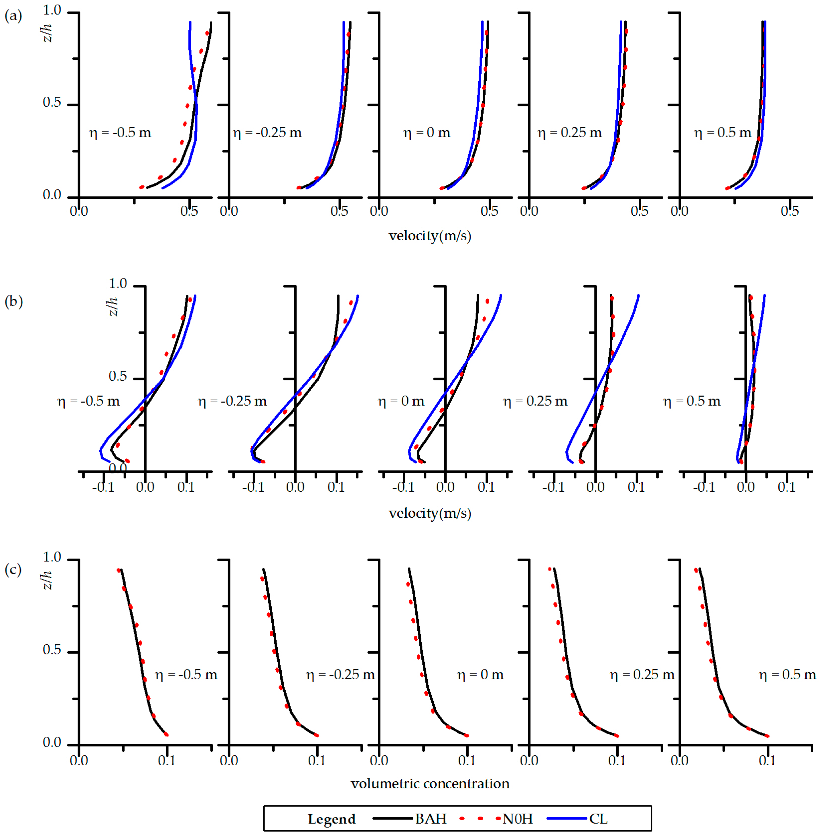
Figure 8 shows the results for the higher concentration case (BAH and N0H) in comparison with the CL case. The secondary flow in the runs BAH and N0H seems weaker than the CL case. Similar to the lower concentration case, the eddy viscosity is reduced because of the sediment stratification effect, but the secondary flow is not strengthened in this case. This indicates that the sediment stratification effect on the suppression of the turbulence is not the key factor. As mentioned above, in the cases BAH and N0H, density is taken as a variable quantity in Equation (11). The buoyant force from the sediment stratification effect in the transversal momentum equation controls the secondary flow behavior. For example, consider the profile at centerline (η = 0) in Figure 8. The sediment concentration is larger close to the inner bank and transversal gradient of sediment concentration is very large. Transversal buoyant force direction is outward which is in opposite direction to the transversal surface gradient and the total transversal pressure gradient is smaller. The centrifugal force and the resultant transversal velocity are smaller than the clear water case. Run BAH and N0H have almost the same transversal surface gradient which has decisive role on the total transversal pressure gradient in the upper depth. Run N0H has smaller density in the upper depth compared to BAH. Therefore, in run N0H, the transversal velocity is larger at the upper part of the depth; and accordingly, the transversal surface gradient becomes larger, thus the transversal velocity in the lower depth increases in the reverse direction. Therefore, the secondary flow in run N0H is stronger than that in run BAH. This means the effect of sediment inertia on the flow momentum is significant while the Boussinesq approximation cannot disclose the flow information at higher concentration in meandering channels.
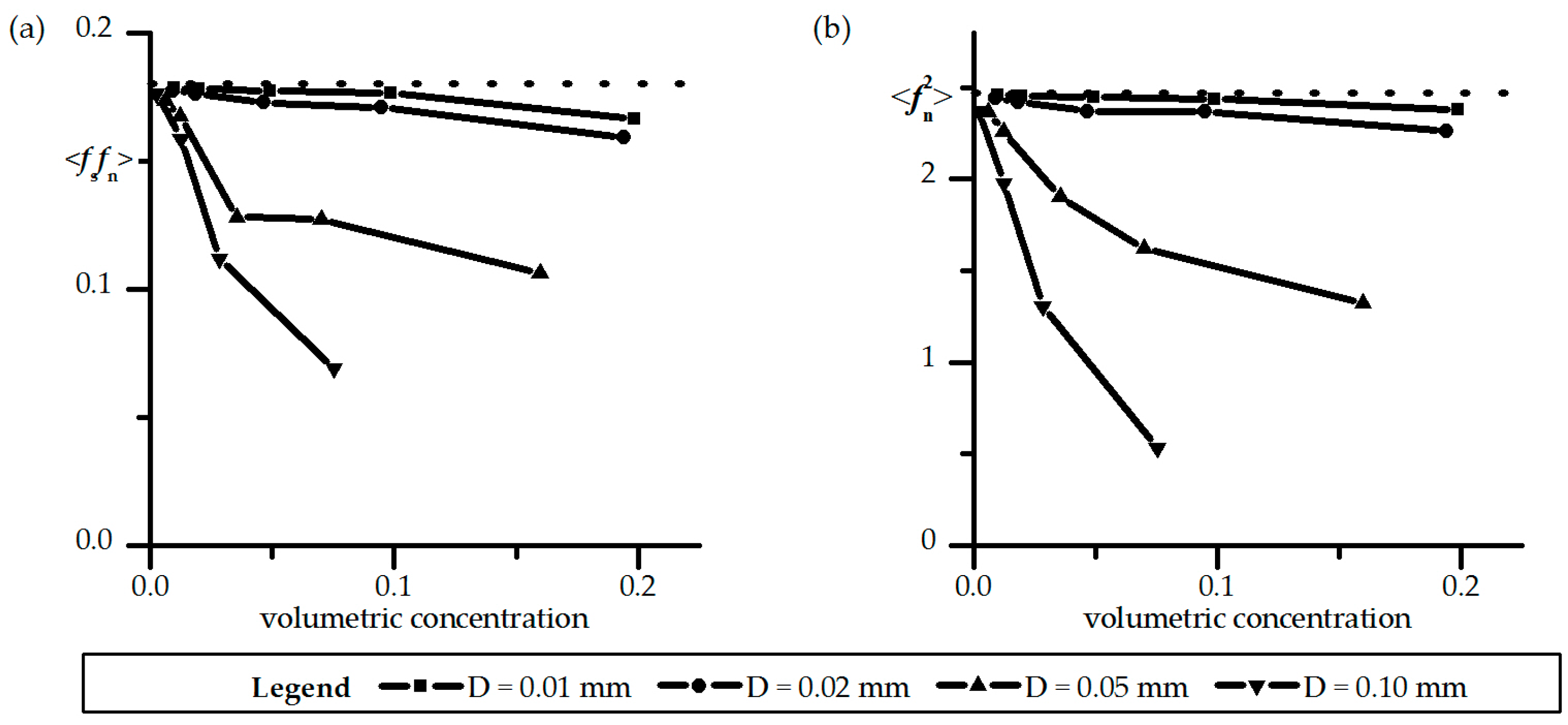
Runs N0H and BAH have higher concentration where sediment inertia effect is equally important as stratification effect. To illustrate the integrated effect on the secondary flow with different concentrations and sediment sizes, the sensitivity analysis on the size and concentration of sediment is discussed here. Two normalized quantities <fn2> and <fsfn> were adapted as characteristic parameters which represent the secondary flow strength and advecting flow momentum [39]. The sediment size is varied from 0.01 to 0.1 mm with depth averaged volumetric concentration from 0.01 to 0.2 at the inlet. The sediment buoyancy effect on turbulence is excluded here as the simple profile presented in Equation (12) for eddy viscosity was employed in this analysis. The results are summarized in Figure 9. The secondary flow strength decreases as the concentration increases. The finer sediment has a nearly uniform profile and only slightly affects the secondary flow strength. For 0.05- and 0.10-mm sediments, the non-uniformity of concentration profile at low concentration is much higher, vertical density gradient is large and the secondary flow strength declines efficiently to ¼ with concentration larger than 0.075. At higher concentration, the group hinder settling velocity is much smaller and the profile approaches to uniformity. Thus, the decrease retards and an exponentially decaying rate is found for the secondary flow here.
4. Conclusions
This paper presents 3D numerical simulations of sediment laden flows in open channel meanders concerning suspension inertia effect on the flow structure. The 3D governing equations without the Boussinesq approximation were used here and both the inertia and buoyant effects were considered. The velocity and concentration calculations performed in bend channels with comparison between the cases with and without Boussinesq approximation. Sediment size and specific density of sediment were studied to demonstrate the integrated effect. Although the additional turbulence transport produced by the presence of sediment could not be simulated by the present model due to the limitations with the employed turbulence closure model, the modifications in the vertical profiles of concentration and velocity due to the sediment were still estimated successfully, similar to the previous studies.
The Boussinesq approximation that neglects all other density effects except buoyancy for dilute flows results in obvious discrepancy in flow structure and sediment transport for high sediment concentration in meandering channels. Both the inertia and stratification effects of sediment play important roles in river meandering processes. The stratification effect promotes secondary flow at lower concentration by reducing eddy viscosity and suppresses secondary flow at higher concentration by the buoyance force acting on transversal pressure. The inertia effect suppresses secondary flow which is important at higher concentration. Depending on the sediment concentration and diameter, the integrated effect results in an increase and a decrease of the secondary flow at lower and higher concentrations, respectively. This suggests that the dominance of the sediment effect depends on the concentration. With the increase of concentration under a specific sediment size, secondary flow increases to reach a maximum and then declines. Moreover, as the sediment concentration rises, an exponentially decaying rate has been found for the secondary flow subject to inertia effect (Figure 9). It is concluded that numerical simulations without considering the Boussinesq approximation is necessary when concentration is high in meandering channels.
The present qualitative predictions based on the 3D numerical simulations provide a new perspective on sediment laden flow. A quantitative analysis of the inertia and stratification performance in meandering channels provides a comprehensive understanding of the water-sediment interactions. The lower Yellow River carries a heavy sediment load with bed material mainly composed of fine sand and silt. The main stream channel migrates very fast during the occurrence of hyperconcentrated flows while the meandering mechanics is still an open question. Extensive research efforts, including numerical modelling, have been continuously carried out on meandering mechanisms. Highly efficient 2D models are still the main tools for river engineering and perform quite satisfactorily in straight or mild meandering rivers [40]. This study would give some cues to 2D and 3D modelling of fluvial process for sediment laden flows.
Author Contributions
Funding acquisition, writing—review, project administration and supervision, X.S. X.F. and E.K.; methodology, software, validation, and writing—original draft preparation, F.Y. and X.F.
Funding
This research was funded by National Key R&D Program of China (Grant No. 2018YFC0407402) and National Natural Science Foundation of China (NSFC, Grant Nos. 51525901 and 91747207).
Conflicts of Interest
The authors declare no conflict of interest. The funders had no role in the design of the study; in the collection, analyses, or interpretation of data; in the writing of the manuscript, or in the decision to publish the results.
References
- Vanoni, V.A. Transportation of Suspended Sediment by Water. Trans. Am. Soc. Civ. Eng. 1946, 111, 67–102. [Google Scholar]
- Einstein, H.A.; Chien, N. Effects of Heavy Sediment Concentration near the Bed on Velocity and Sediment Distribution; University of California, Institute of Engineering Research: Oakland, CA, USA, 1955. [Google Scholar]
- Smith, J.D.; McLean, S.R. Spatially averaged flow over a wavy surface. J. Geophys. Res. 1977, 82, 1735–1746. [Google Scholar] [CrossRef]
- Lyn, D.A. A Similarity Approach to Turbulent Sediment-Laden Flows in Open Channels. J. Fluid Mech. 1988, 193, 1–26. [Google Scholar] [CrossRef]
- Valiani, A. An open question regarding shear flow with suspended sediments. Meccanica 1988, 23, 36–43. [Google Scholar] [CrossRef]
- Castro-Orgaz, O.; Giráldez, J.V.; Mateos, L.; Dey, S. Is the von Kármán constant affected by sediment suspension? J. Geophys. Res. Earth Surf. 2012, 117. [Google Scholar] [CrossRef]
- Turner, J.S. Buoyancy Effects in Fluids; Cambridge University Press: New York, NY, USA, 1973. [Google Scholar]
- Styles, R.; Glenn, S.M. Modeling stratified wave and current bottom boundary layers on the continental shelf. J. Geophys. Res. Oceans 2000, 105, 24119–24139. [Google Scholar] [CrossRef] [Green Version]
- Lamb, M.P.; D’Asaro, E.; Parsons, J.D. Turbulent structure of high-density suspensions formed under waves. J. Geophys. Res. Oceans 2004, 109. [Google Scholar] [CrossRef]
- Taylor, P.A.; Dyer, K.R. Theoretical models of flow near the bed and their implications for sediment transport. Sea 1977, 6, 579–601. [Google Scholar]
- Herrmann, M.J.; Madsen, O.S. Effect of stratification due to suspended sand on velocity and concentration distribution in unidirectional flows. J. Geophys. Res. 2007, 112. [Google Scholar] [CrossRef]
- Nezu, I.; Azuma, R. Turbulence Characteristics and Interaction between Particles and Fluid in Particle-Laden Open Channel Flows. J. Hydraul. Eng. 2004, 130, 988–1001. [Google Scholar] [CrossRef]
- Wright, S.; Parker, G. Density Stratification Effects in Sand-Bed Rivers. J. Hydraul. Eng. 2004, 130, 783–795. [Google Scholar] [CrossRef]
- Muste, M.; Yu, K.; Fujita, I.; Ettema, R. Two-phase versus mixed-flow perspective on suspended sediment transport in turbulent channel flows. Water Resour. Res. 2005, 41. [Google Scholar] [CrossRef]
- Winterwerp, J.C. Stratification effects by fine suspended sediment at low, medium, and very high concentrations. J Geophys. Res. Oceans 2006, 111. [Google Scholar] [CrossRef]
- Winterwerp, J.C. Stratification effects by cohesive and noncohesive sediment. J Geophys. Res. Oceans 2001, 106, 22559–22574. [Google Scholar] [CrossRef] [Green Version]
- van Maren, D.S.; Winterwerp, J.C.; Wu, B.S.; Zhou, J.J. Modelling hyperconcentrated flow in the Yellow River. Earth Surf. Process. Landf. 2009, 34, 596–612. [Google Scholar] [CrossRef]
- Byun, D.S.; Wang, X.H. The effect of sediment stratification on tidal dynamics and sediment transport patterns. J. Geophys. Res. Oceans 2005, 110. [Google Scholar] [CrossRef]
- Amoudry, L.O.; Souza, A.J. Impact of sediment-induced stratification and turbulence closures on sediment transport and morphological modelling. Cont. Shelf Res. 2011, 31, 912–928. [Google Scholar] [CrossRef] [Green Version]
- Cantero, M.I.; Balachandar, S.; Parker, G. Direct numerical simulation of stratification effects in a sediment-laden turbulent channel flow. J. Turbul. 2009, 10. [Google Scholar] [CrossRef]
- Ozdemir, C.E.; Hsu, T.J.; Balachandar, S. A numerical investigation of fine particle laden flow in an oscillatory channel: The role of particle-induced density stratification. J. Fluid Mech. 2010, 665, 1–45. [Google Scholar] [CrossRef]
- Cantero, M.I.; Shringarpure, M.; Balachandar, S. Towards a universal criteria for turbulence suppression in dilute turbidity currents with non-cohesive sediments. Geophys. Res. Lett. 2012, 39. [Google Scholar] [CrossRef]
- Dutta, S.; Cantero, M.I.; Garcia, M.H. Effect of self-stratification on sediment diffusivity in channel flows and boundary layers: A study using direct numerical simulations. Earth Surf. Dyn. 2014, 2, 419–431. [Google Scholar] [CrossRef]
- Dallali, M.; Armenio, V. Large eddy simulation of two-way coupling sediment transport. Adv. Water Resour. 2015, 81, 33–44. [Google Scholar] [CrossRef]
- Cao, Z.; Wei, L.; Xie, J. Sediment-laden flow in open channels from two-phase flow viewpoint. J. Hydraul. Eng. 1995, 121, 725–735. [Google Scholar] [CrossRef]
- Zhong, D.; Zhang, L.; Wu, B.; Wang, Y. Velocity profile of turbulent sediment-laden flows in open-channels. Int. J. Sediment Res. 2015, 30, 285–296. [Google Scholar] [CrossRef]
- Liang, L.; Yu, X.; Bombardelli, F. A general mixture model for sediment laden flows. Adv. Water Resour. 2017, 107, 108–125. [Google Scholar] [CrossRef]
- Chauchat, J.; Cheng, Z.; Nagel, T.; Bonamy, C.; Hsu, T.-J. SedFoam-2.0: A 3D two-phase flow numerical model for sediment transport. Geosci. Model Dev. Discuss. 2017, 10, 1–42. [Google Scholar] [CrossRef]
- Zeytounian, R.K. Joseph Boussinesq and his approximation: A contemporary view. Comptes Rendus Mécanique 2003, 331, 575–586. [Google Scholar] [CrossRef]
- Kundu, P.K.; Cohen, I.M. Fluid Mechanics; Elsevier: Amsterdam, The Netherlands, 2008; p. 297. [Google Scholar]
- Lin, B.; Roger, A.F. Numerical modelling of three dimensional suspended sediment for estuarine and coastal waters. J. Hydraul. Res. 1996, 34, 435–456. [Google Scholar] [CrossRef]
- Wu, W. Computational River Dynamics; CRC Press: Boca Raton, FL, USA, 2007; p. 297. [Google Scholar]
- Warner, J.C.; Sherwood, C.R.; Arango, H.G.; Richard, P.S. Performance of four turbulence closure models implemented using a generic length scale method. Ocean Model. 2005, 8, 81–113. [Google Scholar] [CrossRef]
- Yeh, T.; Cantero, M.; Cantelli, A.; Pirmez, C.; Parker, G. Turbidity current with a roof: Success and failure of RANS modeling for turbidity currents under strongly stratified conditions. J. Geophys. Res. Earth Surf. 2013, 118, 1975–1998. [Google Scholar] [CrossRef] [Green Version]
- Zhang, Y.; Baptista, A.M.; Myers, E.P. A cross-scale model for 3D baroclinic circulation in estuary–plume–shelf systems: I. Formulation and skill assessment. Cont. Shelf Res. 2004, 24, 2187–2214. [Google Scholar] [CrossRef]
- Coleman, N.L. Effects of suspended sediment on the open-channel velocity distribution. Water Resour. Res. 1986, 22, 1377–1384. [Google Scholar] [CrossRef]
- Wang, Z.B.; Ribberink, J.S. The validity of a depth-integrated model for suspended sediment transport. J. Hydraul. Res. 1986, 24, 53–67. [Google Scholar] [CrossRef]
- Blanckaert, K. Saturation of curvature-induced secondary flow, energy losses, and turbulence in sharp open-channel bends: Laboratory experiments, analysis, and modeling. J. Geophys. Res. Earth Surf. 2009, 114. [Google Scholar] [CrossRef]
- Blanckaert, K.; de Vriend, H.J. Nonlinear modeling of mean flow redistribution in curved open channels. Water Resour. Res. 2003, 39. [Google Scholar] [CrossRef]
- Pu, J.H.; Hussain, K.; Shao, S.; Huang, Y. Shallow sediment transport flow computation using time-varying sediment adaptation length. Int. J. Sediment Res. 2014, 29, 171–183. [Google Scholar] [CrossRef] [Green Version]
Figure 1.
Equilibrium condition: estimated profiles of velocity (a) and sediment concentration (b) in comparison with the experimental data.
Figure 1.
Equilibrium condition: estimated profiles of velocity (a) and sediment concentration (b) in comparison with the experimental data.

Figure 2.
Non-equilibrium condition: calculated sediment concentration profiles in comparison with the experimental data.
Figure 2.
Non-equilibrium condition: calculated sediment concentration profiles in comparison with the experimental data.

Figure 3.
Plan view of Blanckaert’s laboratory flume.

Figure 4.
Distribution of the depth-averaged streamwise velocity: (a) Experiment; (b) modelling.

Figure 5.
Calculated streamwise velocity profiles in comparison with the measurements: (a) Cross-section 90°; (b) cross-section 180°. η is the position in the lateral direction from the central line towards the outer bank.
Figure 5.
Calculated streamwise velocity profiles in comparison with the measurements: (a) Cross-section 90°; (b) cross-section 180°. η is the position in the lateral direction from the central line towards the outer bank.

Figure 6.
Calculated transverse velocity profiles in comparison with the measurements: (a) Cross-section 90°; (b) cross-section 180°. η is the position in the lateral direction from the central line towards the outer bank.
Figure 6.
Calculated transverse velocity profiles in comparison with the measurements: (a) Cross-section 90°; (b) cross-section 180°. η is the position in the lateral direction from the central line towards the outer bank.

Figure 7.
Velocity and sediment concentration profiles at the cross-section 90° for lower concentration case: (a) Streamwise velocity; (b) transversal velocity; (c) sediment volumetric concentration. (velocity unit: m/s).
Figure 7.
Velocity and sediment concentration profiles at the cross-section 90° for lower concentration case: (a) Streamwise velocity; (b) transversal velocity; (c) sediment volumetric concentration. (velocity unit: m/s).

Figure 8.
Velocity and sediment concentration profiles at the cross-section 180° for higher concentration case: (a) Streamwise velocity; (b) transversal velocity; (c) sediment volumetric concentration. (velocity unit: m/s).
Figure 8.
Velocity and sediment concentration profiles at the cross-section 180° for higher concentration case: (a) Streamwise velocity; (b) transversal velocity; (c) sediment volumetric concentration. (velocity unit: m/s).

Figure 9.
<fn2> and <fsfn> variation with suspended sediment at the center of cross-section 90°. The dot line represents the clear water (CL) case.
Figure 9.
<fn2> and <fsfn> variation with suspended sediment at the center of cross-section 90°. The dot line represents the clear water (CL) case.


Table 1.
Conditions of numerical simulations.
| Run | BAL | N0L | CL | BAH | N0H |
|---|---|---|---|---|---|
| D (mm) | 0.05 | 0.05 | - | 0.05 | 0.05 |
| Boussinesq approximation | Yes | No | - | Yes | No |
| cb | 0.015 | 0.015 | 0 | 0.10 | 0.10 |
| ρs/ρw − 1 | 1.65 | 1.65 | - | 1.65 | 1.65 |
© 2019 by the authors. Licensee MDPI, Basel, Switzerland. This article is an open access article distributed under the terms and conditions of the Creative Commons Attribution (CC BY) license (http://creativecommons.org/licenses/by/4.0/).
Share and Cite
MDPI and ACS Style
Yang, F.; Shao, X.; Fu, X.; Kazemi, E. Simulated Flow Velocity Structure in Meandering Channels: Stratification and Inertia Effects Caused by Suspended Sediment. Water 2019, 11, 1254. https://doi.org/10.3390/w11061254
AMA Style
Yang F, Shao X, Fu X, Kazemi E. Simulated Flow Velocity Structure in Meandering Channels: Stratification and Inertia Effects Caused by Suspended Sediment. Water. 2019; 11(6):1254. https://doi.org/10.3390/w11061254
Chicago/Turabian StyleYang, Fei, Xuejun Shao, Xudong Fu, and Ehsan Kazemi. 2019. "Simulated Flow Velocity Structure in Meandering Channels: Stratification and Inertia Effects Caused by Suspended Sediment" Water 11, no. 6: 1254. https://doi.org/10.3390/w11061254
Note that from the first issue of 2016, this journal uses article numbers instead of page numbers. See further details here.