Assessing the Impacts of Best Management Practices on Nonpoint Source Pollution Considering Cost-Effectiveness in the Source Area of the Liao River, China

Abstract

Agricultural nonpoint source pollution has been a major influential factor on the deterioration of water quality in the Liao River source area. Best management practices (BMPs), as a comprehensive pollution prevention system designed to reduce the impacts of agricultural activities and improve water quality, has been considered one of the most effective solutions for nonpoint source pollution control. However, economic cost has been an important element for screening the implementation of BMPs. Both pollution reduction and capital expenditure need to be resolved with the actual situation. A water quality model such as the Soil and Water Assessment Tool (SWAT) and empirical cost algorithm are important tools to assess the cost-effectiveness of the effects of BMPs on nonpoint source pollution. In this study, BMP scenarios including buffer strips (BSs), fertilizer reduction (FR), forest land increase (FLI), grassland increase (GLI), and their combination were implemented using the SWAT model; furthermore, the efficiency of their pollutants reduction and costs benefit were estimated in the watershed. The results showed that combined BMPs have better control effects than a single BMP, with “BS20 (widths 20 m) + FR15 (fertilization reduction 15%) + FLI (forest land increase)” arriving at the greatest loads reduction in the critical periods. From environmental and economic perspectives, the cost-effectiveness of interception measures is higher than that of the source control measures. The results indicated that BS was the most environmentally friendly practice, and FR was the most economically efficient out of all the BMPs. Regarding land-use changes, FLI was more environmentally friendly, and GLI was more economically efficient. The most economical and effective BMPs can be designated as follows: BS1.5 (widths 1.5 m) and FR15 (fertilization reduction 15%). Therefore, due to possible differences in government policies, it is important to consider an integrated approach for all the relevant actors and seek sustainable environmental and economic development.

1. Introduction

Agricultural nonpoint source pollution (ANPS) has caused widespread concern and attention due to the need for effective control of point source pollution [1]. In agricultural activities, excessive pesticide and fertilizer application will lead to nutrient leaching and soil erosion, resulting in the loss of nonpoint source pollution increasing constantly. The United States Environmental Protection Agency (USEPA) has reported that 44% of water quality was deteriorated in United States in the 21st century [2]. The main reason is that excessive nutrients enter the river, causing distinct degrees of eutrophication. In European countries, nonpoint source pollution has become the primary factor in water pollution [3]. In China, the situation of agricultural nonpoint source pollution is also not optimistic; nitrogen and phosphorus pollution load accounts for more than 50% in the water bodies, and ANPS has become the main cause of water environment problems in the watershed [4].

Nowadays, with the increasing prevalence of ANPS in China, the large-scale nonpoint source pollution that first occurred in the warm southern regions has been extended to the cold northern regions [5]. China’s northeast regions are affected by the climatic conditions; the winter is cold and long, leading to the migration and transformation of nonpoint source pollution in particular. The winter freezing–thawing phenomenon promotes the mineralization of pollutants, and a large amount of nitrogen and phosphorus are accumulated in the soil [6]. In early spring, the melt of snowfalls causes a severe snowmelt runoff scouring effect, and initiates concentrate outflows of nonpoint source pollutants during the snow melting period. Therefore, it’s an important challenge to research the control of ANPS, due to its accumulation and sudden appearance in the cold regions.

Among the measures to reduce ANSP, the best management practices (BMPs) have proven to be the most effective methods to control ANSP [7]. The implementation of BMPs is an approach that aims to improve water quality based on the pollution control theory of “source reduction–interception–repair”. At present, since the primary purpose of BMPs is to reduce pollutants, the most important studies in China have focused on the environmental benefits of BMPs’ implementation, but few studies have assessed the cost-effectiveness of the measures, despite the cost of BMPs limiting their practical implementation [8]. Stewart simulated the reduction of nonpoint source pollution by returning farmland to grassland, and found that TN (total nitrogen) and TP (total phosphorus) loads in the watersheds decreased by 31% and 36%, respectively [9]. Liu investigated the effectiveness of seven BMP scenarios on ANSP reduction in the Three Gorges Reservoir; the results indicated that reducing the local fertilizer level should obtain a satisfactory environmental and economic efficiency [10]. However, there are two important concerns about the environment and economy that need to be considered and managed at the same time. Marcelo selected alternative crop, buffer strips, and fertilization reduction as BMPs and estimated the pollutant reduction effect and costs benefit for the Treene catchment, Germany [11]. Furthermore, some researchers discovered that a single BMP often fails to meet the needs of water quality control objectives in cold climatic conditions regions; however, the proposal of a reasonable set of combined BMPs implementation will greatly contribute to controlling ANSP [12,13].

Assessment of the control efficiency of BMPs is a key step in determining whether a measure is applicable. There are many studies that have showed the effectiveness of ANSP based on site monitoring before and after different BMPs implementation [14,15]. However, this approach takes a long time and requires extensive measurements; as a result, most research studies gradually transformed into hydrological model simulations. The Soil and Water Assessment Tool (SWAT) has been used widely to predict flow, sediment, and nonpoint source pollution loads at large-scale watershed [16]. Meanwhile, multiple studies have applied SWAT by modifying the parameters inside the model to estimate the impact of BMPs on water quality [17]. Panagopoulos applied the sensitivity analysis method to identify the SWAT model internal parameters corresponding to different no-tillage, irrigation, fertilization, contour planting, etc., in the Arachtos watersheds, and realized the simulation of different reduction measures [18]. Haas used water quality models to predict the reduction rates of river discharge and nitrate loads, while developments in BMP optimization strategies have further improved the feasibility of implementing BMPs on large watersheds [19]. In this way, these studies confirmed the suitability of the SWAT model for investigating the potential reduction of pollutants for different BMPs; the assessment can be considered both ecological and economic [20].

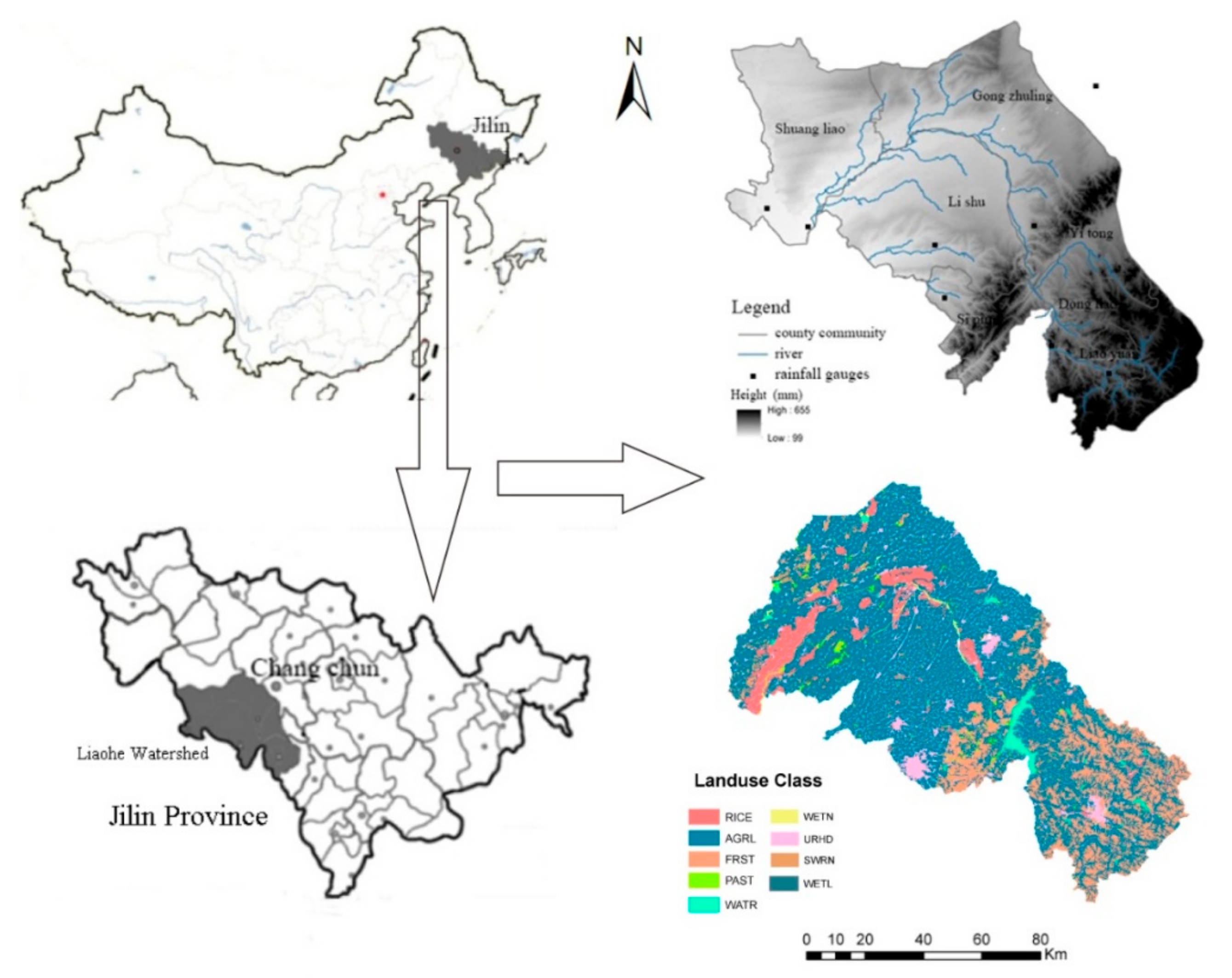
The Liao River source area is located in the cold region of northeast China, where unique climate conditions and frequent agricultural activities lead to serious problems with ANPS. The changes of land use and fertilization management are major factors affecting runoff and nonpoint source pollution in the study area. This study attempts to use the SWAT model to analyze the spatial–temporal distribution of nitrogen and phosphorus pollution annually and during the snowmelt period in the source area of Liao River, and assess the efficiency of BMPs and their combination in reducing ANSP while considering cost expenditure during the precipitation and snowmelt periods, respectively. Ultimately, it will identify the cost-effectiveness of best management practices for the environment and the economy. Based on these purposes, the research can contribute to improving water quality regarding agricultural watershed and aid in making decisions for reducing pollution with the best management practices in the Liao River source area.

2. Study Area and Data

2.1. Study Area

The Liao River source area is a typical cold area that is located in the southwest of Jilin Province (123°43′–125°32′ E, 42°36′–44°18′ N) in China, with the elevation ranges from 112 to 622 meters (Figure 1). The area of the Liao River watershed is about 11,283 km² and includes three subbasins, which are the Liao River basin, the Zhaosutai River basin, and the Tiaozi River basin. The average precipitation is about 520 mm/year (1961–2012), of which 80% occurs from June to September. The average temperature is 5.4 °C/year with the lowest value of −14.8 °C in January. The freeze–thaw period lasts for 120–150 days of each year. Frozen soil is usually from late October to early May, and the maximum freeze depth is 130–150 cm [21].

The land use in the watershed is mainly agricultural; about 60% is covered by farmland (dry fields and paddy field). The main crops are corn and rice. Annually, approximately 677,000 tons of fertilizers (nitrogen application rate up to 300 kg/hm²) are used for agricultural production in the Liao River source area, exceeding the internationally recognized upper limit of nitrogen application (225 kg·hm⁻²). As an important issue in the study area, the daily average TN and TP loads presented 8.79 t/d and 0.65 t/d for the period of 2006 to 2010. The precipitation runoff period (summer) presented 6.97 t/d nitrate loads and 0.49 t/d phosphorus loads, while the snowmelt runoff period (spring) presented 1.12 t/d and 0.13 t/d [22]. The mitigation of nonpoint source pollution caused by agricultural activities is of great importance for water quality deterioration in the watershed. In order to solve environmental problems, it is necessary to assess the impacts best management practices on ANPS in the Liao River source area.

2.2. Data Input

The major data input for this study were acquired by material collection, and include a digital elevation model (DEM) from the national DEM of China with a resolution of 90 m × 90 m, land-use database from Landsat TM (thematic mapper) and ETM (enhanced thematic mapper) image data in 2008, and soil property database from the second soil survey in Jilin Province. Daily weather data (maximum/minimum temperatures, precipitation, wind speed, relative humidity, and solar radiation) were obtained from the China Meteorological Data Sharing Service Network in the period from 2000 to 2010 [23]. Runoff, sediment, and nonpoint source pollution input data were provided by five meteorological stations and three hydrological stations, which are located at Changchun, Siping, Shuangliao, Liaoyuan, Erlongshan Reservoir, Quantai, Wangben, and Lishu, as shown in Figure 1.

In this study, the fertilizer and pesticide application management for crops were in view of feedback from local farmers and governmental agencies. The main crops in the study area include corn (planting area 90%), rice (planting area 7%), and wheat (planting area 3%). The fertilizers used mainly include urea and NPK (nitrogen phosphorus and potassium) compound fertilizers, etc. The amount of fertilizer applied to rice is far greater than the amount applied to corn. Based on this information, we focused on nitrogen and phosphorus fertilization for two main crops, which are corn and rice. The crops are only planted once a year. The fertilizer management was considered regarding the average applied amount of nitrogen and phosphorus for corn (128 kg·N·ha⁻¹ and 42 kg·P·ha⁻¹) and rice (166 kg·N·ha⁻¹ and 54 kg·P·ha⁻¹) every year. The fertilization time of rice is about 10 days after transplanting, and corn is about 10 to 15 days after sowing, usually in May; then, there is additional fertilization in July.

3. Methodology

The study is according to the technology route process in Figure 2. Firstly, the improved SWAT model is set up, calibrated, and validated by considering sensitivity analysis on the snowmelt parameters of snow melting module; then, the model is applied to assess the impacts on TN and TP loads under three BMPs. Furthermore, all the BMPs are evaluated with two criteria, TN and TP loads reduction and costs of implementation.

3.1. SWAT Model

The SWAT model was developed by Arnold at the United States Department of Agriculture [24]. It is a semi-distributed model based on a physical mechanism that simulates hydrology processes, sediment transport, and pollutant loads for different land-use management and agriculture practices at variable scale basins for extended periods of time. An important capability of the SWAT model is to provide a scenario analysis module that is suitable for the prediction and assessment of management measures such as BMPs. It modifies the default generated mgt. file through the user interface and enters generalized information on various measures into the model [25]. In this way, the SWAT model has been widely used to research changes in various management measures.

In 2002, a snow melting module has been added to the SWAT model by Fontaine, which extends it from the southern warmer regions to the northern cold regions in China [26]. In our study, seven snowmelt parameters in the SWAT snow melting module were analyzed to describe the sensitivity of the model, and the optimum value range of snowmelt parameters were determined through the sensitivity analysis method. The results show that five snowmelt parameters including SFTMP (snowfall temperature), SMTMP (snowmelt temperature), SMFMX (maximum snowmelt factor), SMFMN (minimum snowmelt factor), and TIMP (snowpack temperature gag factor) were considered sensitive, while SNOCOVMX (minimum snow water content that corresponds to 100% snow cover) and SNO50COV (fraction of SNOCOVMX that corresponds to 100% snow cover) were considered insensitive. The best range of both SMFMX and SMFMN varied from 18 to 20 mm H₂O·°C⁻¹·d⁻¹ and from 6 to 8 mm H₂O·°C⁻¹·d⁻¹, while SMTMP and SFTMP varied from −20 to 20 °C, and TIMP varied from 0 to 0.1. The detailed description for snowmelt parameters sensitivity analysis method can be found in our published paper [27].

3.2. Best Management Practices

Best management practices (BMPs) are an effective policy aimed at improving the water environment resulting from agricultural activities. It has been widely used for the control of soil erosion and nonpoint source pollution [28,29]. Several impact factors such as the land-use changes, soil types and slopes, essential pollution zones, project implementation cycle timing, and locations will influence the beneficial results of BMPs on water quality and economic costs. For example, a buffer strip is a BMP that is located riverside, while fertilizer management is direct in the field. Therefore, it is important to understand the geographical and spatial–temporal distribution of nonpoint source pollution in the watershed in order to choose the suitable BMPs implementation on each area.

Due to the long-term monitoring on field measurement methods, the model simulation has become a common choice to evaluate nonpoint source pollution reduction after BMPs implementation in a large-scale watershed, and widely used in long-term or short-term effect evaluations [30]. In this study, the BMPs implemented were represented in the SWAT model by modified reduction measures simulation factors and parameters in SCS-CN (soil conservation service curve number) runoff modules and soil modules. According to a previous literature review and the local agricultural background in the Liao River source area, three BMPs were selected: buffer strip, fertilization reduction, and forest and grassland increase. In addition, due to the unique climatic conditions in cold regions, the disparities of measures during precipitation runoff and snowmelt runoff periods should also be considered. In this way, the efficiency of each BMP and their combination regarding nitrogen and phosphorus loads reduction and costs were assessed based on the differences between the current simulation values and the values after the implementation of BMPs. Therefore, the BMPs in different scenarios at precipitation and snowmelt periods could be simulated successively in the SWAT model as follows.

3.2.1. Buffer Strip (BS)

Buffer strips (BSs) are important measures that utilize vegetation zones to remove sediment and nonpoint source pollution from surface runoff through percolation, infiltration, and adsorption [31]. The effectiveness of buffer strips depends on many factors, including the vegetation type and composition, soil type, pollution location, slope, and width [32]. In this study, the soil type is mainly chernozem and flat farmland with a slope of 0 to 5° in the source area of the Liao River. It is suitable for constructing vegetation buffer zones on both sides of the riverine; the plant species are bushes and arbors. Based on previous different research considering pollutants reduction, six practical variations of BS widths were tested to evaluate the effects on nitrogen and phosphorus loads reductions, namely 1.5 m (BS1.5), 3 m (BS3), 5 m (BS5), 10 m (BS10), 15 m (BS15), and 20 m (BS20). For this survey, the BSs widths are operated by modifying the parameter FILTERW in SWAT. The BSs were applied to all the essential pollution zones, and compared relationships between pollution reduction efficiency and buffer strip width for hydrological response unit (HRU9, HRU12, HRU25, and HRU28) in different slopes with agriculture activities.

3.2.2. Fertilizer Reduction (FR)

Due to fertilizer being the main source of agriculture nonpoint source pollution, the most effective and essential way to depress NSP is to reduce fertilization use. Fertilizer reduction is one of the most commonly implemented BMPs; several studies have indicated the benefits of this practice [33,34]. These studies showed that different methods can be adopted to reduce fertilizer, which included examples of utilizing biological fertilizer instead of traditional fertilizer. In addition, sprayer technologies can be applied to increase fertilizer availability and reduce the amount of applied fertilizer. However, it is difficult for these approaches to achieve results in practice due to complicated impact factors in technology transfers and spatial effect in large-scale use. In this study, based on previous reference and realistic requirements in the study area, the effects of three different fertilizer reduction rates regarding nitrogen and phosphorus loads were assessed: 5% (FR5), 10% (FR10), and 15% (FR15) of the current use amount [35,36]. The FRs were suitable for all the crops. The fertilization replacement amount can be set up within an .mgt file in the SWAT.

3.2.3. Forest and Grassland Increase (FLI/GLI)

Forest and grassland increase (FLI/GLI) is a planned and step-by-step approach to stop sloping farmland that is liable to cause soil erosion, and restore forests and grasses based on local conditions, thereby decreasing agricultural activities [37]. The relevant regulations require that cultivated fields in steep sloping farmland on both sides of the river source and around the lake and reservoir—as well as ecologically important areas with soil erosion and sandstorm hazards seriously—should be returned to forests and grasses that are prioritized in the plan (State Council Order from the People’s Republic of China, 2003) [38]. In this study, sloping farmland accounts for 60% of the total cultivated fields, and the gradient ranges from 3° to 15° in the northeast. Sloping farmland is mainly concentrated in the midstream and downstream in the Liao River source area; at the same time, this area is also an essential pollution zone. Therefore, the hydrologic response units (HRUs) HRU2, HRU5, HRU6, HRU7, HRU9, HRU12, HRU13, HRU25, HRU26, HRU27 and HRU28 (in the middle and lower stream) are selected for returning farmland to forests and grasslands. Two scenarios were considered to assess the effects on nitrogen and phosphorus loads reductions: forest land increase (FLI) and grassland increase (GLI) for all the essential pollution zones. According to the cultivated area with a slope of more than 5°, the new land uses were implemented in the SWAT model with increasing the forests or grasses by 30% of the essential pollution sloping farmlands.

3.2.4. Combination of the BMPs

BMPs may attain higher efficiency when implemented in combination. The combined pattern of various BMPs was simulated in the SWAT model. For this research, the combination of the above three management measures were applied by modifying the module parameters, in order to further study nitrogen and phosphorus pollutants reduction and implementation costs in the watershed.

Table 1. Best management practices (BMPs) names and signs.

BMP Name	Sign
Buffer strip 1.5 m	BS1.5
Buffer strip 3 m	BS3
Buffer strip 5 m	BS5
Buffer strip 10 m	BS10
Buffer strip 15 m	BS15
Buffer strip 20 m	BS20
Fertilization reduction 5%	FR5
Fertilization reduction 10%	FR10
Fertilization reduction 15%	FR15
Forest land increase	FLI
Grassland increase	GLI

summarized all the abbreviations of individual BMPs that will be used in the following sections.

3.3. BMP Costs

In addition to the nitrogen and phosphorus reduction under the premise of meeting environmental governance requirements, the economic costs of BMPs also need to be evaluated as an important factor in choosing nonpoint source pollution control measures [39,40]. The costs estimation in this study considered the implementation, installation, and maintenance expenditure for BS, FLI, and GLI, as well as market revenue for land-use changes (FLI and GLI) and FR. The implementation and installation costs generally include an expense of pre-project construction, management, labor force, and scientific research, et al. The costs of maintenance are essential for programs as important as implementation/installation costs. It represents the subsequent protection costs after the implementation of BMPs. Moreover, these costs are greatly variable in different periods and region conditions. The market revenue reflects the profitability of crops and is used primarily to assess the crop implementation. It expresses the declining income from the changes in land use such as arable land loss and crop yield reduction due to less fertilization. The income loss value is calculated through the area (ha) occupied by FLI/GLI or FR multiplying by the crop productivity (t/ha), and then multiplying by the current crops market prices (€/t) for commissariat. However, these values are not always stable, because the crops production and market prices may vary with different factors such as climatic conditions. In this study, the costs for the BMPs implementation was obtained by empirical calculation based on references and Social Economic Yearbook in Jilin Province for 2016–2017. The costs are given in Euros (1000 €) for a better comparative. Lam indicated that the calculated cost for the BMP is a general reference value, as the factors may be changed and the characteristics may vary in different watersheds [41].

The cost-effectiveness analysis is a commonly evaluation tool for BMPs that is designed to meet the lowest costs of combined measures under water quality conditions or maximize water quality under a certain cost constraint. In the study, the simulated pollution loads reduction was divided by the calculated costs of each BMP; the result is taken as the cost-effectiveness value (CE). The higher the CE, the better cost-effectiveness of the BMP, meaning more loads reduction with lower costs and easier adoption by decision makers. The calculation formula is as follows:

$$\mathrm{CE}=\frac{\mathrm{Loads} \mathrm{reduction} \left(\mathrm{t}\right)}{{\mathrm{Costs}}_{-}\mathrm{Total} \left(€\right)}$$

(1)

Among them, CE means cost-effectiveness value; Loads reduction represents the difference in pollution loads before and after the implementation of BMPs; Costs_Total represents the coupled between the initial implementation/installation costs and income losses.

In this way, we assessed the effectiveness of BMPs implementation by the maximization of the ratio between nonpoint source pollution loads reduction and total costs for the Liao River source watersheds.

4. Results and Discussion

4.1. SWAT Model Calibration and Validation

The watershed was divided into 37 hydrologic response units (HRUs) in the SWAT. The LH-OAT (Latin hypercube one factor-at-a-time) sensitivity analysis was carried out 24 parameters that were identified as having an influence on flow, sediment, and nonpoint source pollution [42], as shown in

Table 2. Sensitivity analysis results of parameters in the calibrated and validated model.

Parameters	File	t-Start	p-Value	Parameters	File	t-Start	p-Value
CN2	mgt	12.74	0	SMFMN	bsn	−0.49	0.63
SOL_K	sol	−10.64	0	SURLAG	bsn	0.46	0.66
CANMX	hru	2.56	0.01	EPCO	hru	0.35	0.73
ALPHA_BF	gw	2.27	0.026	TIMP	bsn	−0.26	0.79
ESCO	hru	1.84	0.07	REVAPMN	gw	−0.24	0.81
SMFMX	bsn	1.83	0.07	SFTMP	bsn	0.22	0.82
BIOMIX	mgt	−1.13	0.26	USLE_P	mgt	26.31	0.00
GWQMN	gw	1	0.32	SLSUBBSN	hru	14.73	0.00
SOL_Z	sol	−0.98	0.33	SPCON	bsn	−1.42	0.16
SMTMP	bsn	−0.88	0.38	SPEXP	bsn	0.48	0.63
CH_K2	rte	−0.83	0.41	HRU_SLP	hru	0.43	0.67
SOL_AWC	sol	−0.5	0.62	USLE_C	crop	0.07	0.94

. Among these parameters, the most sensitive parameters were CN2, SOL_K, CANMX, ALPHA_BF, and ESCO for flow, as well as USLE_P and SLSUBBSN for sediment. In addition, we compared simulation results with consideration of snowmelt parameters (SFTMP, SMTMP, SMFMX, SMFMN, TIMP) or not during the snow melting period (November to April). The detailed evaluation results can be found in our published papers [27]. It shows that considerable snowmelt parameters can improve the accuracy for the snowmelt process.

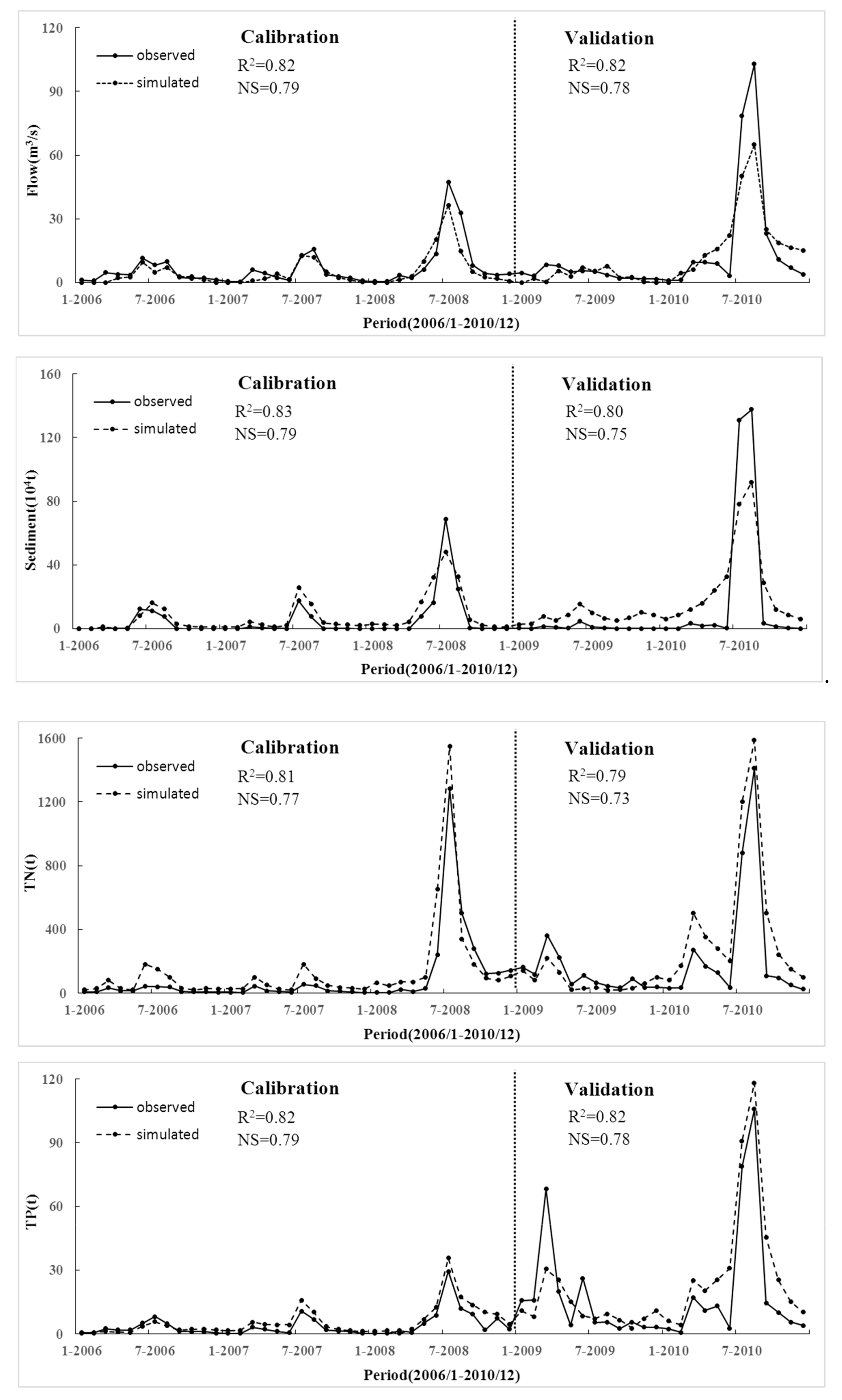
The daily flows, sediment, TN data, and TP data from 2006 to 2010 that were obtained from Quantai station were selected for model calibration and validation with using the optimum value range of snowmelt parameters and other parameters. The calibration period was 2006 to 2008, and the validation period was 2009 to 2010. Graphs of observed and simulated values for monthly average daily flows, sediment, TN loads, and TP loads in the calibration and validation periods are shown in Figure 3. It shows that the simulated results meet the accuracy requirements, of which R² ≥ 0.6 and NS ≥ 0.5; the SWAT model considering the snowmelt module was able to simulate flow, sediment, nitrogen, and phosphorus loads at the watershed outlet.

4.2. Spatial–Temporal Distribution of TN and TP Loads

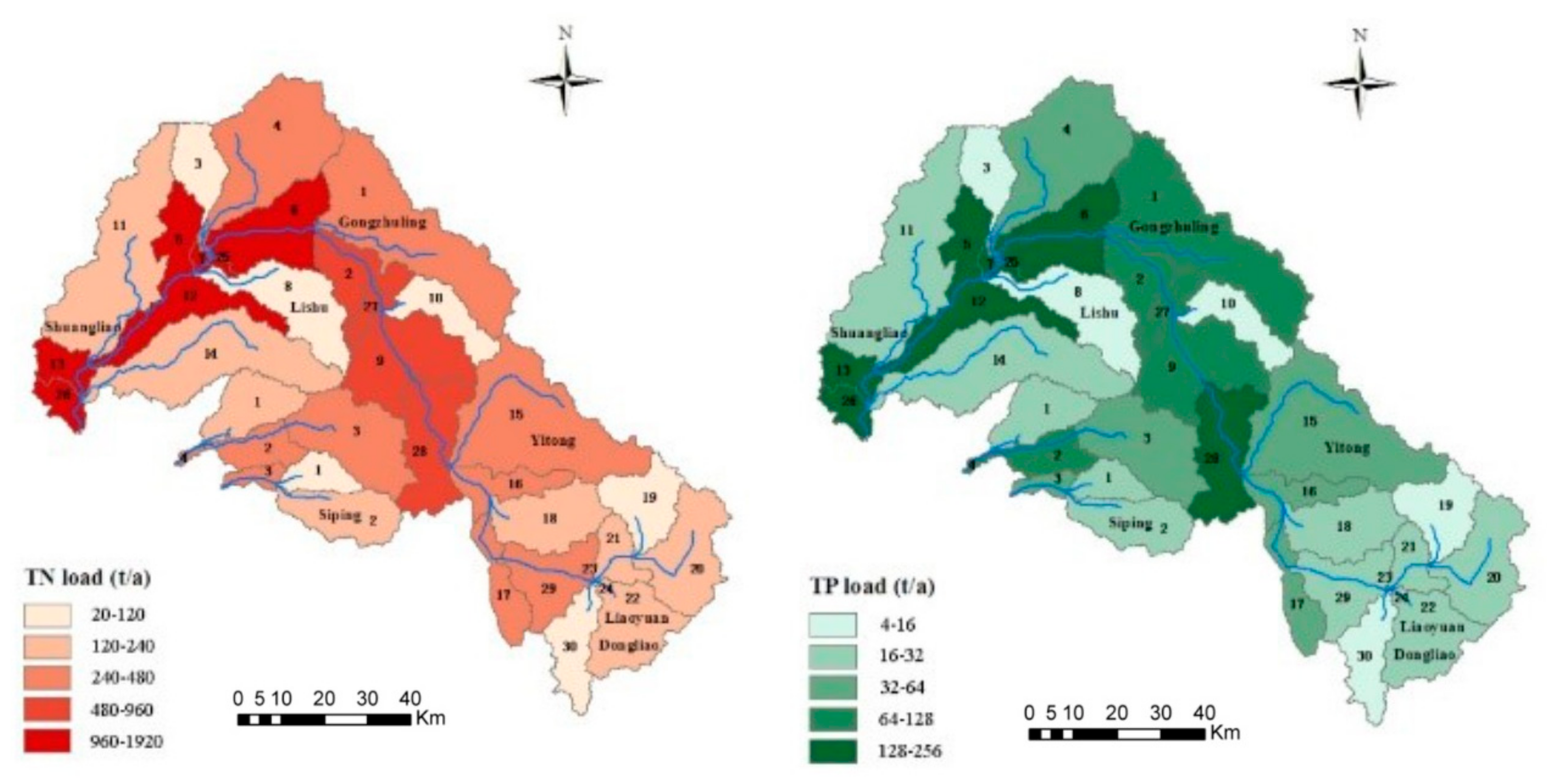
Agricultural activities such as the excessive application of fertilizers and pesticides have significant effects on the nonpoint source pollution. Figure 4 is the spatial distribution of TN and TP loads for a general situation in 2010. It indicates the essential pollution zones that provide the contributions of nonpoint source pollutant exports, including HRU2, HRU5, HRU6, HRU7, HRU9, HRU12, HRU13, HRU25, HRU26, HRU27, and HRU28. These areas are mainly farmland with strongly agricultural activities, excess fertilization, livestock and poultry breeding, and an intensively rural population distribution, which leads to serious pollutant losses.

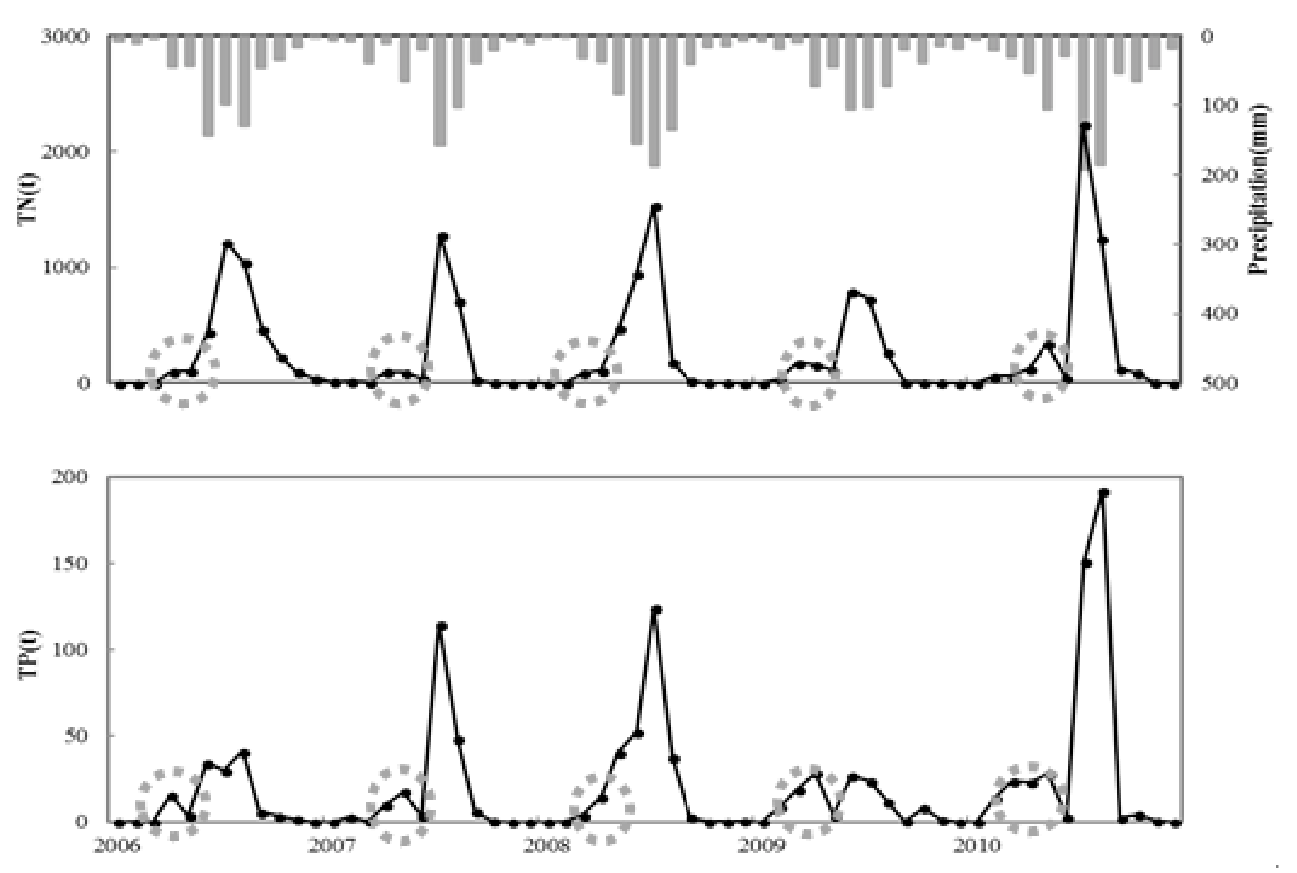
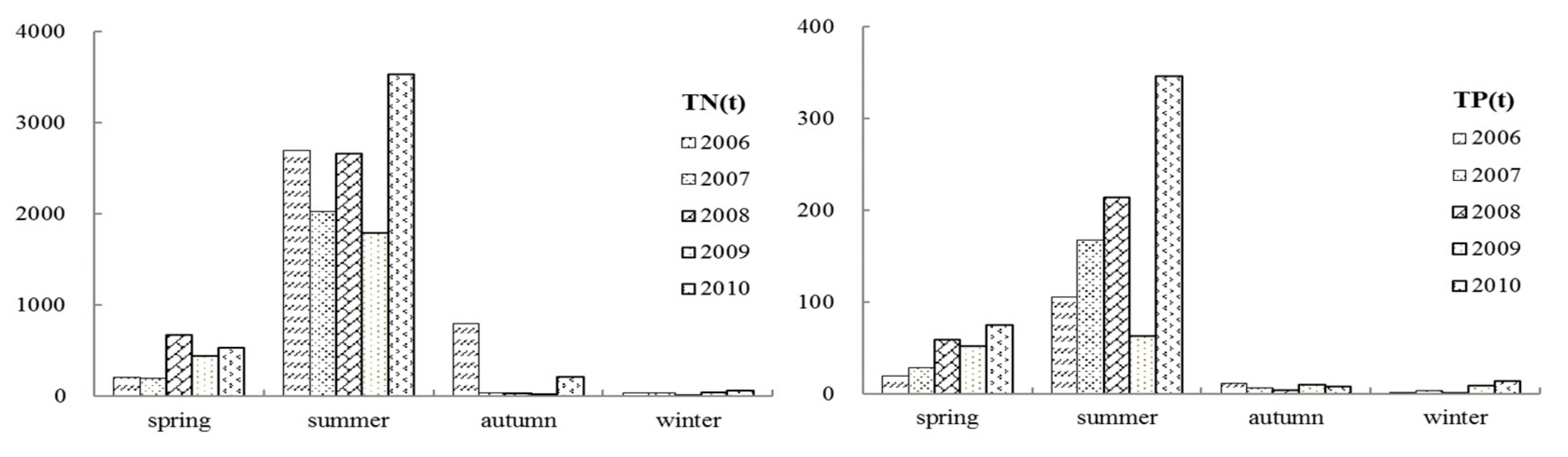
The temporal characteristics of TN and TP loads were also simulated for time series 2006 to 2010, as shown in Figure 5. The outputs of TN and TP have almost the same change trend to precipitation in the study area, with two peaks focused on July to September and March to May (as seen in gray circled) every year. In order to analyze the high-risk period and driving factors of nonpoint source pollution, Figure 6 gives the average seasonal TN and TP loads during five years as well as the proportion in each season. It shows that nonpoint source pollution outputs are mainly concentrated in the summer, followed by spring. The average proportion of TN and TP loads accounted for 75.12% and 79.42% in the summer, as well as 17.28% and 14.74% in the spring, respectively. With the intensive agricultural activities, the higher precipitation in summer is the main reason for the large amount of pollutants leaching to the river. In addition, as the study area is located in cold regions, which has a long freezing period each year, both TN and TP loads will accumulate and become very high in the spring due to the snow melting accompanied by a severe snowmelt runoff flushing effect, resulting in pollutant losses concentrated in a short period of time. Therefore, snowmelt is the driving force for the occurrence of nonpoint source pollution in the spring. In summary, the temporal and spatial distribution of nonpoint source pollutants loads has certain seasonal particularity, especially during the precipitation runoff period (summer) and the snowmelt runoff period (spring) in the source area of the Liao River.

4.3. Simulation of BMPs

As described in the literature [43], the effects of BMPs implementation are diverse. In generally, the implementation of BMPs confirmed reductions on TN and TP loads at the watershed outlet. In this study, as the particularity of spatial–temporal distribution on nonpoint source pollution in the study area, the BMPs projects were performed in one year, and the pollutant reductions efficiency was analyzed in a precipitation runoff period (summer) and snowmelt runoff period (spring) respectively as follows.

4.3.1. Buffer Strip Management

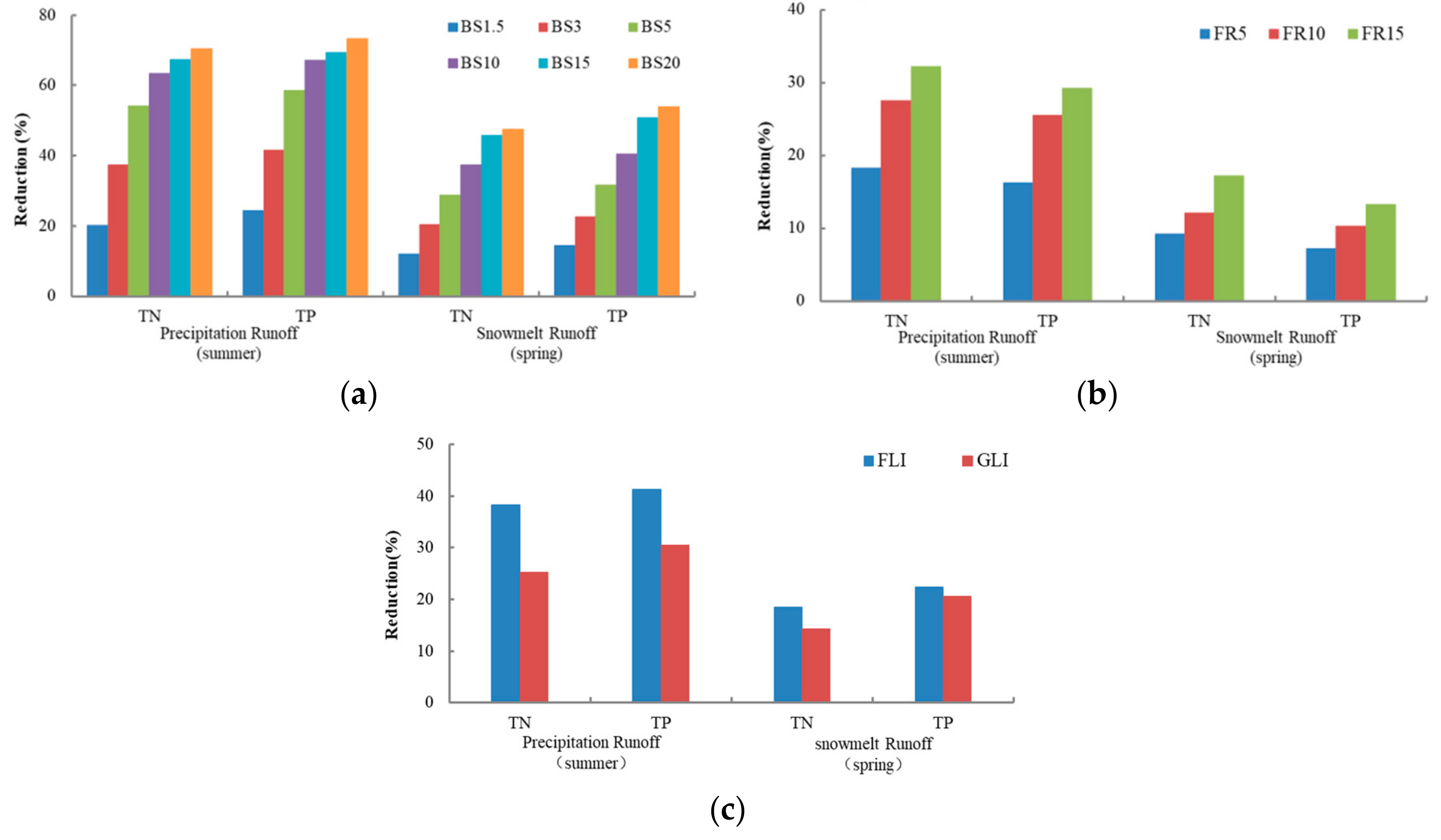
The BS simulation presented the highest effective reduction of TN and TP loads at the essential pollution zones. Figure 7a showed the evaluation of loads reduction with different buffer widths. The BS1.5, BS3, BS5, BS10, BS15, and BS20 indicated 12.12–20.16%, 20.37–37.45%, 28.75–54.12%, 37.34–63.48%, 45.75–67.43%, and 47.44–70.54% TN loads reduction per year in precipitation runoff and snowmelt runoff periods, as well as 14.38–24.45%, 22.52–41.64%, 31.64–58.56%, 40.43–67.21%, 50.78–69.34%, 53.85–73.23% TP loads reduction. It illustrated that the reduction efficacy of TN and TP loads increase quickly with buffer width, while the rate of increase gradually decreases as the buffer becomes wider, until BS10 in the precipitation runoff period and BS15 in the snowmelt runoff period. Meanwhile, the reduction rate in the precipitation runoff period is higher than that in the snowmelt runoff period. It means that a greater effectiveness of BSs occurred in the summer, which had a larger runoff presence due to precipitation and higher load peaks, since the greater plant can effectively absorb and intercept pollutions to leach in this period. Moreover, there is a higher reductions efficiency of TP compared with TN under the same BS width. This is because soluble phosphorus is more easily lost with runoff and erosion than soluble nitrogen.

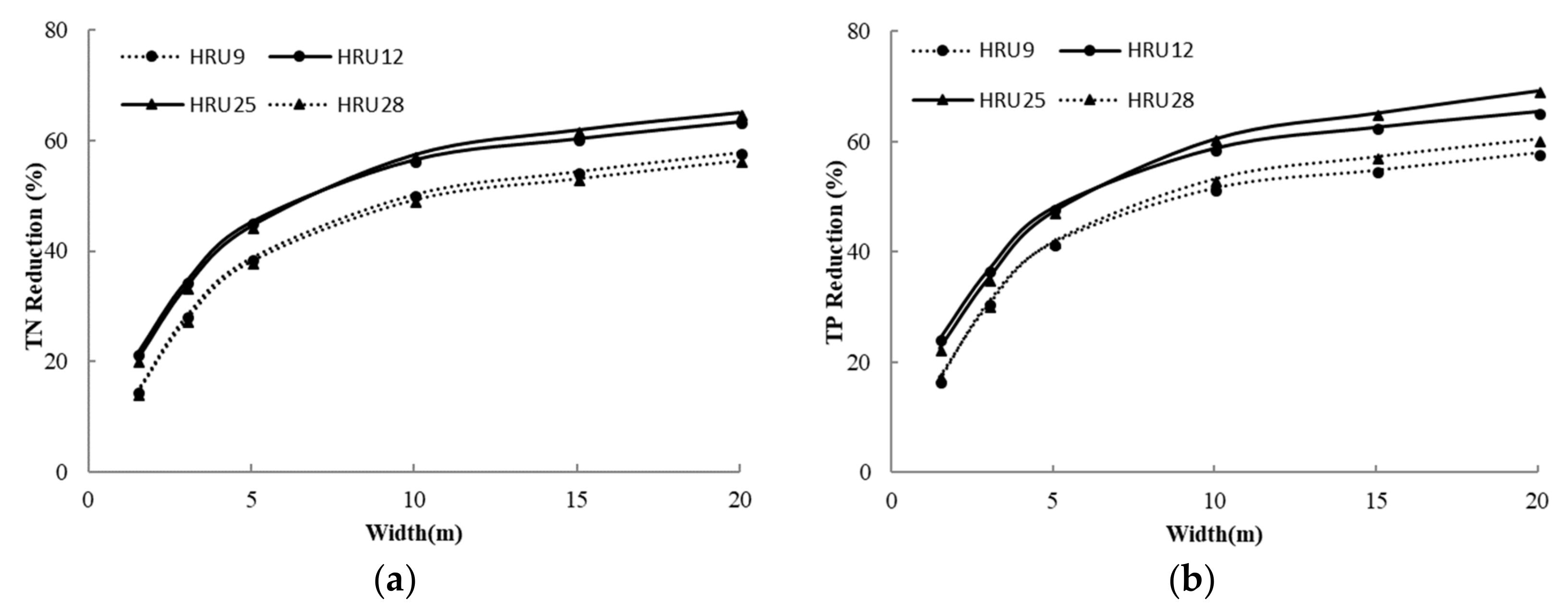
Figure 8 shows the relationship between the buffer strip width and pollutions reduction efficiency for TN and TP in four HRUs with different slopes. Among them, HRU9 and HRU28 are steeper than HRU12 and HRU25. All of these HRUs simulations illustrate that the increase in BS width will lead to higher pollutions reduction. However, for the same BS width, the units with relatively steeper slopes (HRU9 and HRU28) had lower pollutant reductions efficiency than the units with flatter slopes (HRU12 and HRU25).

4.3.2. Fertilizer Management

The simulations of TN and TP loads reduction with FR were significant at the watershed outlet. The FR results of loads reduction efficiency are showed in Figure 7b. A fertilization rate reduction by 5% (FR5) led to a decrease TN and TP loads of 9.25–18.23% and 7.38–16.47% in the precipitation runoff and snowmelt runoff periods, the reduction by 10% (FR10) represented less 12.11–27.47% and 10.31–25.47%, as well as less 17.45–32.33% and 13.84–29.46% pollution loads reaching the river by 15% reduction (FR15), respectively. The percentage of loads reduction increases as fertilizer use decreases in all the phases, for both the precipitation runoff and snowmelt runoff periods. Summer presented the highest reductions, which was due to the excessive application of fertilizers during the previous farming period in the study area, once the large decrease in fertilizers results in a significant reduction in nonpoint source pollutants for being transported with precipitation runoff entering the river. For the spring snowmelt period, the accumulated nitrogen and phosphorus in the soil also decreased, leading to loads reduction for leaching with snowmelt runoff, but obviously lower than that in the summer. Furthermore, the TN reduction greatly improved compared with TP when fertilizer application was reduced. This is because TP is sedimentary, the utilization rate of phosphate fertilizer is low, and the annual application is not effective, leading to TP being deposited and accumulating in the soil year by year. Therefore, the reduction effect of TP takes a long time to appear. However, due to the negative charge of nitrate, it can’t be absorbed by soil particles and can be easily moved by surface runoff. Thus, the accumulation of TN is not as strong as TP, so the reduction of TN is more effective than that of TP.

In addition, FRs may also cause a reduction in crop yields. There is a direct correlation between fertilizer application and crop yields. Marcelo et al. (2017) concluded that crop production drops by 13% and 10% when the fertilization rate is reduced by 15% for corn and pasture, and drops by 26% and 20% when the fertilization rate is reduced by 30%. The above studies have indicated that crops will present an average reduction that is double or even stronger when fertilizers are reduced by different percentages. In this study, FR5, FR10, and FR15 would lead to reductions of 5%, 10%, and 15% on all the crop yields, respectively.

4.3.3. Land-Use Management

The simulation results of the SWAT model showed that the increase in forest and grassland areas has little impact on pollutants reduction in the watershed. Figure 7c showed the results regarding the reduction efficiency of TN and TP loads with FLI and GLI. FLI led to a reduction of TN and TP loads of 18.56–38.24% and 22.43–41.35%, while the pollution loads of GLI only decreased 14.23–25.25% and 20.54–30.45% in the precipitation runoff and snowmelt runoff periods. Theoretically, land-use changes can lead to higher reductions because the soil is covered by forests and grasslands as well as the lower fertilization. However, changes to only 30% of the essential pollution zones—representing only 2.8% of the watershed—couldn’t significantly affect the TN and TP loads. Despite all this, the effect of reduction was highest in the precipitation runoff period. This result showed evidence that the existence of forests and grasses increase nitrogen and phosphorus uptake by lush plants and less surface runoff and soil erosion in this period. Moreover, when forest and grass areas are increased, the reduction of TP was much greater than that of TN. This is because soluble phosphorus attached to the sediment particles, which were easy to be transferred in runoff; decreased soil erosion can significantly reduce this part of phosphorus loss.

This study also found that the reduction efficiency of TN and TP loads by returning farmland to forests is greater than returning farmland to grasslands. This is because the canopy storage and interception capacity of forests is stronger, and the soil water storage capacity is larger.

Another factor is due to the strong and networked forest rooting systems, which will be firmly entangled with the soil, thus achieving the purpose of consolidating soil. Thereby, when precipitation runoff occurs, the forests have a better sand-fixing effect and stronger soil and water conservation capacity than grassland.

4.3.4. Combined BMPs

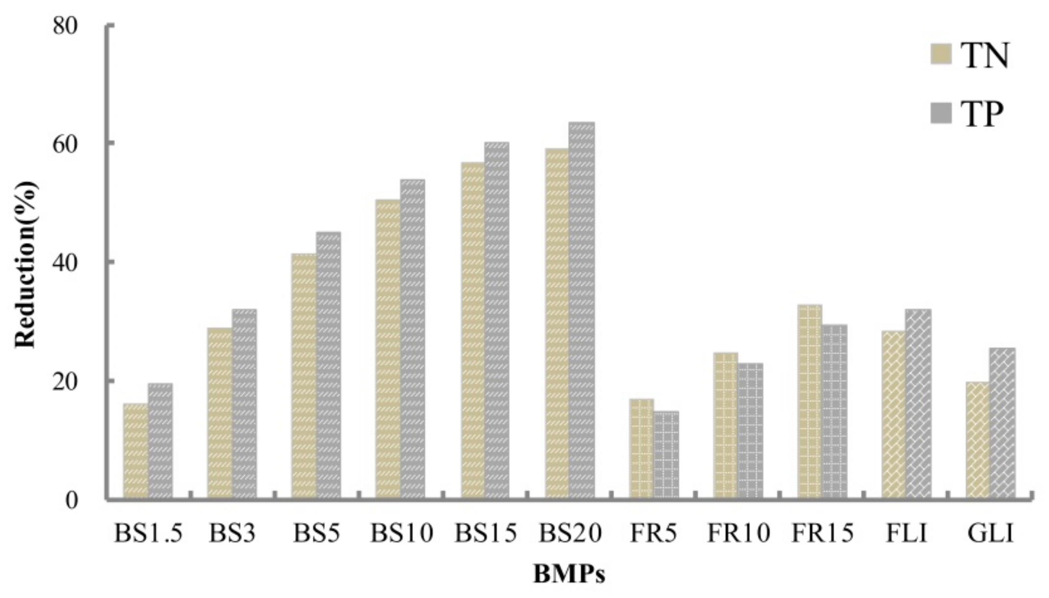
The comprehensive evaluation on TN and TP loads reduction of each BMP is shown in Figure 9. It can be seen from the above research that the reduction effect of buffer strip is much better than that of returning farmland to forests or grasses and fertilizer reduction management. However, each BMP will influence different nitrogen and phosphorus transportation processes in the watershed, such as more storage in the soil, more vegetable absorption, as well as less infiltration and loss. However, due to the cumulative response of TN and TP, the effect of forest or grassland increase and fertilizer reduction management is slower, but it is a source control measure that is necessary to improve water quality in the long term. On the contrary, the buffer strip has the best effect, because it adopts the method of directly intercepting pollutants, and it is an important measure to quickly improve the water quality of the watershed.

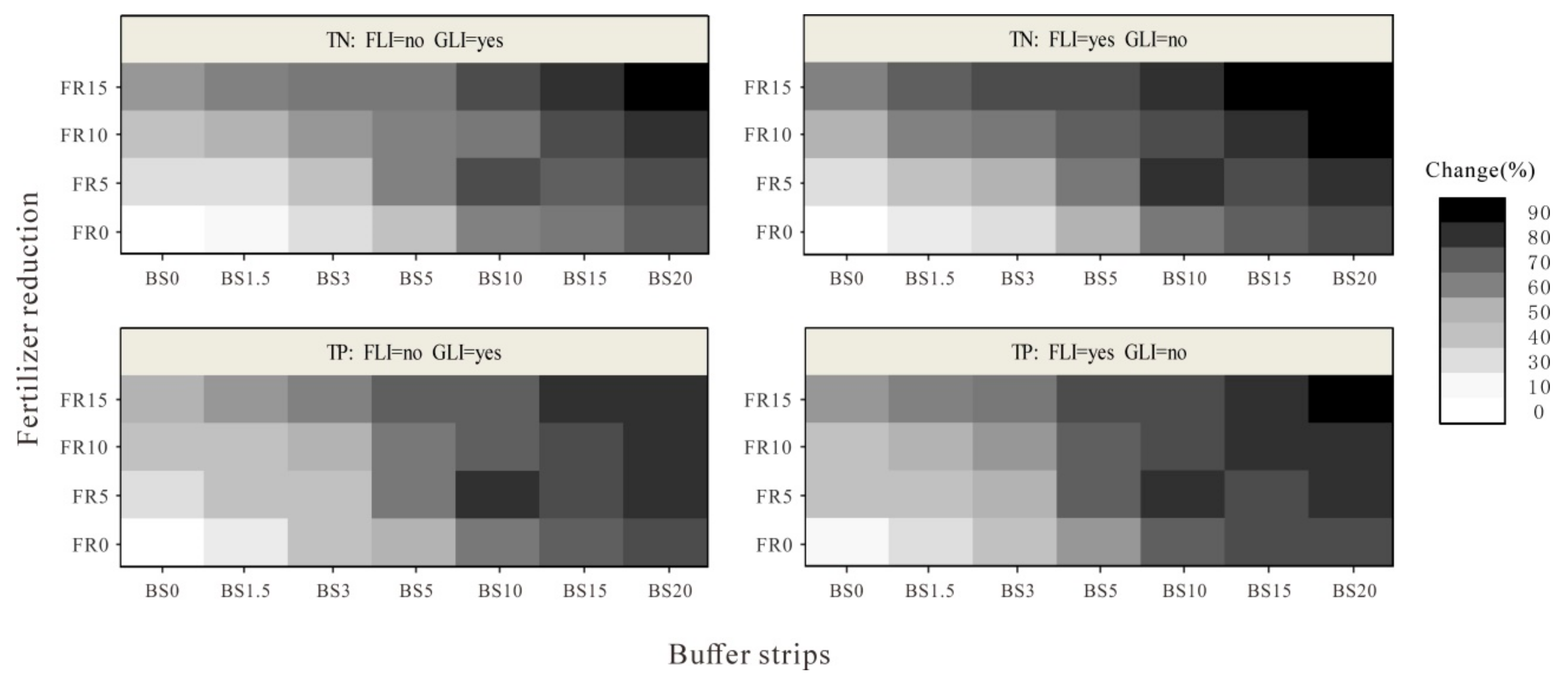
Afterwards, the BMPs were combined to assess TN and TP loads reduction in the SWAT model that is caused by more than one BMP simultaneously. In the simulation, all the possible combinations were presented and experimented until all the BMP implementations were combined with each other; the results are shown in Figure 10.

Through comprehensive management measures, the combined BMPs showed reductions of 18.75–88.62% of the TN loads and 20.45–85.33% of the TP loads. The lowest reduction was combined by “BS1.5” + “GLI”, and the highest reduction was “BS20” + “FR15” + “FLI”. It showed that the positive effect was obtained from different BMPs combinations complementing each other, which means that the more BMPs that were combined together, the more the TN and TP loads were reduced correspondingly. The significant trend of the combined BMPs simulation found that the appearance of BS20 causes the best results with respect to the reduction of TN and TP loads. However, BS width was important, since BS10 presented a relatively high reduction rate. Actually, there was a quick loads reduction rate before the implementation of BS10 (Figure 10, the color shade of the first four columns in the small plots changes quickly); afterwards, the reduction rate is declined (Figure 10, the color shade of the last three columns in the small plots changes slowly). The existence of FR15 also led to better reductions of TN and TP loads, so there is a 15% reduction of fertilizer application, which emerged in the case of relatively high load reductions (Figure 10, first line in small plots). Then, a decaying order was presented in the reduction sequence when FR10 (Figure 10, second line in small plots) and FR5 (Figure 10, third line in small plots) were implemented. The lowest reductions of TN and TP loads in combination appeared without decreasing fertilization (Figure 10, fourth line in the small plots). The application of FLI and GLI also contributed to TN and TP pollutant reductions. Especially, FLI contributions were greater than GLI when comparing the combinations with FLI (Figure 10, top right big box) and the combinations with GLI (Figure 10, top left big box), which was determined by the two important factors of forest canopy interception and forest root systems. Therefore, returning farmland to the forests and grasses had brought an important optimistic effect on nitrogen and phosphorus pollution reduction. Moreover, due to the reduction of pollutants mainly depending on interception activity, the reduction effect of TP is slightly better than TN when observing the combinations almost without FR (Figure 10, third and fourth line in the small plots of top left big box and the bottom left big box). However, when comparing the combinations with FR, the reduction of TN loads is better than that of TP (Figure 10, first and second line in the small plots of the top left big box and the bottom left big box).

Furthermore, it has been found that different combinations of BMPs may result in an analogous reduction effect. For example, the implementation of “BS20” + “FR10” + “GLI” caused similar results with “BS15” + “FR10” + “FLI”. It is necessary to determine different BMP combinations according to the characteristics of watershed; especially, the appropriate practice can be selected by considering the spatial difference of nonpoint source pollution loads. In fact, although some combinations have similar reductions, it should be emphasized that not all BMPs can be replaced by others. For example, FR can’t substitute for BSs, because their effect processes are completely different. However, attempting to shorten the BS width in a specific combination situation is possible.

In addition, the temporal differences of nonpoint source pollution loads are also a major factor to be considered in determining the BMPs combination, which is mainly affected by the two processes of plant absorption and pollutants migration with runoff. In this study, the unique climatic conditions in cold regions affected the simulation results of BMPs implementation—mainly the existence of precipitation runoff and snowmelt runoff—and the features caused a faster response to BS and the reduction efficiency of FR. According to the above analysis, the simulation of TN and TP reduction for all BMPs and their combinations was greater in the precipitation runoff periods, due to the larger runoff and greater plant growth during this period. Therefore, the different combination of BMPs implementation exhibits higher reductions of nitrogen and phosphorus pollutants, primarily in the most crucial periods.

4.4. Analysis of BMPs’ Cost-Effectiveness

The total costs for BMPs implementation are listed in

Table 3. Total costs of BMPs implementation in 1000 € for the watersheds.

BMPs	Unit Costs (€/ha)		Area (ha)	Total Costs (in 1000 €)
	Implementation Costs	Market Revenue
BS1.5	274	0	282.325	77
BS3	547	0	846.975	463
BS5	821	0	1411.625	1159
BS10	1642	0	2823.25	4635
BS15	2462	0	4234.875	10,428
BS20	3283	0	5646.5	18,539
FR5	−276	62	56,465	−12,084
FR10	−551	123	56,465	−24,167
FR15	−827	185	56,465	−36,251
FLI	2864	178	16,939.5	51,530
GLI	1492	178	16,939.5	28,287

. The table shows the cost in 1000 € for the entire watersheds scale. BSs require relatively little costs of initial implementation and installation, and later maintenance costs are negligible. The buffer strips are arranged around the farmland, and the construction area is 0.5–10% of the farmland area. The implementation cost of the measure is about 267 €/ha, and the installation cost is approximately 7 €/ha each year. In contrast, FLI and GLI presented higher costs. Returning farmland to forests and grasses is the national promotion policy. The state provides appropriate grain subsidies according to the economic losses caused by the approved areas of cultivated land, as calculated at a convert of 0.2 €/kg. Simultaneously, the construction area of the project accounts for 30% of the farmland, the total costs of construction and maintenance are 2864 €/ha and 1492 €/ha, respectively. FR actually saves costs due to the reduction of the fertilization amount. According to relevant data, the rice yields in the study area is about 3701.2 kg/ha, the purchase market price is 0.35 €/kg, and the prices of urea (in terms of N) and superphosphate (P₂O₅) are 0.61 €/kg and 0.94 €/kg. The costs of the fertilizer reduction measures are calculated by the income loss due to the decline in crop yield subtracted by the saving costs from reducing the purchase of fertilization.

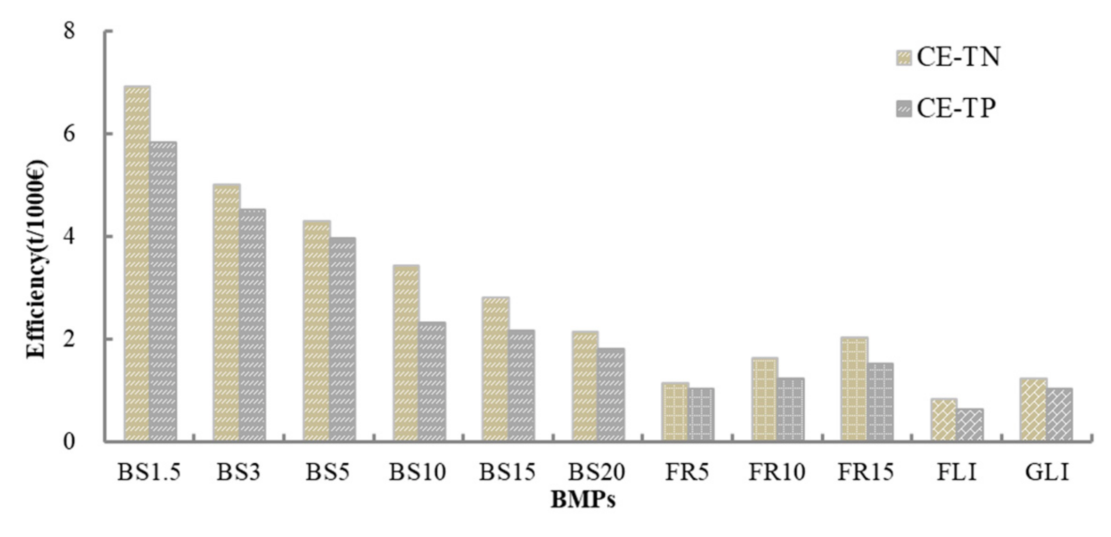
Next, the efficiency of BMPs implementation associated with pollutants reduction and total costs (including implementation, installation, maintenance costs, and market revenue) suggests that this approach is very important for making decisions. Figure 11 illustrated the histogram of CE value with TN and TP; the higher CE value, the better the BMPs’ cost-effectiveness, which means a greater pollutant reduction and thus lower costs.

From the comparison of different scenarios, as the buffer strips width increases during the implementation of BSs, the CE value is lower, which is caused by the increase in cost when the buffer zone expands. In the FRs measure, the CE value of reducing fertilizer by 15% is slightly higher than that by 5%, which may be due to the high fertilization amount in the region. The further reduction of fertilization application has limited impact on crop yield; however, it also reduced the costs of purchasing fertilizer for farmers, so the total cost is lower. Among the land-use change measures, the environmental benefits of FLI are better than those of GLI, but the cost is much higher, resulting in a CE value that is lower than the measures to return farmland to grasslands.

Overall, the cost-effectiveness of interception measures (such as a buffer strip) is higher than that of source control measures (fertilizer reduction and land-use change). In other words, BS was generally the most efficient measure, since it has lower implementation costs and the highest pollution reduction efficiency. It is the best management practice that will be the most suitable for the area and the most acceptable for farmers so far. FR has higher effectiveness due to its nitrogen and phosphorus pollutants reduction and expenses saving, but it also significantly reduced the crop yields, which will lead to a significant loss of income, which may be not easily accepted by farmers. Therefore, the fertilization reduction should be within a certain extent. However, FLI and GLI demonstrated insignificant effectiveness because of the highest implementation costs and the lower pollutants reduction. Despite this, the measure still demands attention because the costs will decrease over the next few years to improve the efficacy; thus, it should be adopted by local governments and farmers in the long term. In any case, although the cost-effectiveness of interception measures is much higher than that of the source control measures, it does not mean that the entire basin only needs to arrange interception measures, the final decisions should be based on the analysis of actual land use, funds status, the social and economic development situation before practical measures are selected for arrangement.

4.5. Multi-Objective Optimization of BMPs

The BMPs discussed in this study are not mutually exclusive, and they can be applied simultaneously. In terms of combining several BMPs, the total costs were considered to be the sum of each cost in principle. This means that the more BMPs that were combined, the higher the costs that were spent (only FR is subtracted). In general, the introduction of FR was a strongly encouraged measure, which could be due to the saving of funds. The effect of combining with BSs will be more prominent, because BSs revealed the best pollutants reduction with reasonable costs for realizing the optimal cost-effectiveness. The efficiency of FR combined with FLI/GLI couldn’t be demonstrated as expected due to the huge implementation cost and income loss. Based on the above analysis, the suggested combination of BMPs for the study area were “BS1.5” + “FR15”. The cost-effectiveness values of the combined BMPs implementation within the watershed were 8.9 kg/€ and 7.3 kg/€ each year. Ultimately, the measures will be in accordance with the collaborative developmental goals for the economy and environment.

5. Conclusions

This study analyzed the cost-effectiveness of BMPs implementation and their impacts on reducing nonpoint source pollution in the source area of the Liao River. The consequence was assessed by using a SWAT model, and the results were simulated under the consideration of two aspects: the environment and the economy.

Initially, a SWAT model considering a snowmelt module could well simulate the spatial and temporal distribution of nonpoint source pollution process in a cold area such as the Liao River watershed. The simulated results indicated the essential pollution zones with different fertilization and land-use types, which meant that spatial differences affected the choice of measures and BMPs that needed to be applied to each area. Likewise, temporal differences were strongly particular and also required measures to meet the specific details of each area. The simulation showed that precipitation and snowmelt are the main driving forces of nonpoint source pollution; in relation, summer and spring are the high-risk seasons. Therefore, the implementation of BMPs in these two periods with the serious pollution issue in the watershed showed a large reduction of nitrogen and phosphorus pollutants.

Furthermore, the reduction effect of TN and TP was evaluated under the different BMPs scenarios, which included source control measures (FR, FLI and GLI) and process control measures (BS). The results of the single measure evaluation show that BSs on the HRU scale had higher efficiency in reducing pollutants than FR, FLI, and GLI, the average reduction rate was as high as 40% and 70% during the spring snowmelt period and the summer precipitation period, respectively, and BSs showed quite different reduction rates in different HRUs, reflecting the important influence of spatial–temporal characteristics on the effectiveness of the interception measures. In addition, a separated measure can’t be sufficient to reduce TN and TP loading significantly; instead, this study reinforced the necessity of combined measures. The results showed that the “BS20 + FR15 + FLI” scenario had the best pollutant reduction effect, and the “BS1.5 + GLI” scenario was limited, which shows the importance of the interception process in nonpoint source pollution control. Therefore, the choice of the best combined BMPs required considering suitable spatial and temporal objectives, so that the combination will have a higher potential for pollutants reduction.

However, it is necessary to consider costs as well as environmental benefit. FR was the most economical of all the BMPs, with the annual benefits saving up to 7.58 × 10⁷ € per year. Followed by BSs; the benefits of BS1.5 were 7.7 × 10⁴ € per year. As for the land-use change practice, FLI was more environmentally friendly, and GLI was more economically efficient. In the cost-effectiveness analysis of BMPs, the CE value of the interception process measures was higher than that of the source control measures. Among them, BS1.5 had the best cost-effectiveness, TN benefits were as high as 6.9 kg/€, and TP benefits were as high as 5.8 kg/€. Meanwhile, FLI had the worst cost-effectiveness; its TN and TP benefits were only 0.81 kg/€ and 0.61 kg/€, respectively. Above all, based on the best pollution loads reduction with reasonable costs, the simulation results suggested that combining BS1.5 and FR15 was the most effective method for the study area, and will satisfy both environmental and economic objectives.

In this way, as an effective approach to control nonpoint source pollution, BMPs play an essential role in pollutants source reduction, process interception, and ecosystem restoration. The choice of BMPs is not only according to the local situation, but also to consider the environmental benefits and economic costs; using water quality model simulation and an empirical cost algorithm to assess the impacts of BMPs can greatly reduce the waste of funds and resources. In addition, this paper highlighted that decision makers should integrate common advice from environmental agencies, administration offices, and farmers alongside BMPs alternatives and more effective agricultural measures to achieve the goals for different demands. In the future, a greater, wider, stronger, and clearer proposal through joint actions is needed to promote economic development with efficient and durable environmental protection programs.

References

1. Lam, Q.D.; Schmalz, B.; Fohrer, N. Assessing the spatial and temporal variations of water quality in lowland areas, Northern Germany. J. Hydrol. 2012, 438, 137–147. [Google Scholar] [CrossRef]
2. Miller, G.T. Living in the Environment: An Introduction to Environmental Science, 7th ed.; Wadsworth Publishing Company: Belmont, CA, USA, 1992. [Google Scholar]
3. Xu, X.; He, P.; Yang, F. Methodology of fertilizer recommendation based on yield response and agronomic efficiency for rice in China. Field Crop. Res. 2017, 206, 33–42. [Google Scholar] [CrossRef]
4. Wang, Y.; Bian, J.M.; Zhao, Y.S. Assessment of future climate change impacts on nonpoint source pollution in snowmelt period for a cold area using SWAT. Sci. Rep. 2018, 8, 2402–2415. [Google Scholar] [CrossRef] [PubMed]
5. Magali, T.; Daniel, C. Evaluating the SWAT’s snow hydrology over a Northern Quebec watershed. Hydrol. Process. 2014, 28, 1862–1871. [Google Scholar]
6. Étienne, L.; François, A.; Ann, V.G. Evaluation of streamflow simulation by SWAT model for two small watersheds under snowmelt and rainfall. Hydrol. Sci. J. 2015, 53, 962–975. [Google Scholar]
7. Ma, X.; Li, Y.; Zhang, M. Assessment and analysis of non-point source nitrogen and phosphorus loads in the Three Gorges Reservoir Area of Hubei Province, China. Sci. Total Environ. 2011, 412, 154–161. [Google Scholar] [CrossRef] [PubMed]
8. Sheshukov, A.V.; Douglas-Mankin, K.R.; Sinnathamby, S. Pasture BMP effectiveness using an HRU-base subarea approach in SWAT. J. Environ. Manag. 2016, 166, 276–284. [Google Scholar] [CrossRef] [PubMed]
9. Stewart, G.R.; Munster, C.L.; Vietor, D.M. Simulating water quality improvements in the Upper North Bosque River watershed due to phosphorus export through turfgrass sod. Trans. ASABE 2006, 49, 257–266. [Google Scholar] [CrossRef]
10. Liu, R.M.; Zhang, P.P.; Wang, X.J. Cost-effectiveness and cost-benefit analysis of BMPs in controlling agricultural nonpoint source pollution in China based on the SWAT model. Environ. Monit. Assess. 2014, 186, 9011–9022. [Google Scholar] [CrossRef]
11. Marcelo, B.H.; Bjorn, G.; Nicola, F. Assessing the impacts of Best Management Practices on nitrate pollution in an agricultural dominated lowland catchment considering environmental protection versus economic development. J. Environ. Manag. 2017, 196, 347–364. [Google Scholar]
12. Li, W.Z.; Li, X.Y. Estimation of the nonpoint source nitrogen load in a strongly disturbed watershed of the North China Plain. Water Sci. Technol. 2014, 69, 1304–1311. [Google Scholar] [CrossRef] [PubMed]
13. David, M.B.; Flint, C.G.; Gentry, L.E. Navigating the socio-bio-Geo-chemistry and engineering of nitrogen management in two LIllinois tile-drained watersheds. J. Environ. Qual. 2015, 44, 368–381. [Google Scholar] [CrossRef] [PubMed]
14. Chen, L.; Qiu, J.; Wei, G. A preference-based multi-objective model for the optimization of best management practices. J. Hydrol. 2015, 520, 356–366. [Google Scholar] [CrossRef]
15. Epelde, A.M.; Cerro, I.; Sanchez-Perez, J.M. Application of the SWAT model to assess the impact of changes in agricultural management practices on water quality. Hydrol. Sci. J. 2015, 60, 825–843. [Google Scholar]
16. Arnold, J.G.; Fohrer, N. SWAT2000: Current capabilities and research opportunities in applied watershed modeling. Hydrol. Process. 2005, 19, 563–572. [Google Scholar] [CrossRef]
17. Liu, M.; Lu, J. Predicting the impact of management practices on river water quality using SWAT in an agricultural watershed. Desalin. Water Treat. 2015, 54, 2396–2409. [Google Scholar] [CrossRef]
18. Panagopoulos, Y.; Makropoulos, C.; Mimikou, M. Reducing surface water pollution through the assessment of the cost-effectiveness of BMPs at different spatial scales. J. Environ. Manag. 2011, 92, 2823–2835. [Google Scholar] [CrossRef]
19. Haas, M.B.; Guse, B.; Pfannerstill, M. A joined multi-metric calibration of river discharge and nitrate loads with different performance measures. J. Hydrol. 2016, 536, 534–545. [Google Scholar] [CrossRef]
20. Xu, X.H.; Tang, Z.H.; Wu, J.F. Preparation and freeze-thaw resistance of alumina based ceramic insulators for extremely cold areas. Ceram. Int. 2017, 43, 2712–2719. [Google Scholar] [CrossRef]
21. Zhao, J. Simulation Research for Export of Agricultural Nonpoint Source Nitrogen and Phosphorus and Its Risk Assessment in the Source Area of Liao River. Ph.D. Thesis, Jilin University, Changchun, China, 2014. [Google Scholar]
22. Wang, Y.; Bian, J.M. Predicting precipitation on nonpoint source pollutant exports in the Source Area of the Liao River, China. Water Sci. Technol. 2016, 74, 876–887. [Google Scholar] [CrossRef]
23. China Meteorological Data Sharing Service Network. Available online: http://cdc.cma.gov.cn/home.do (accessed on 26 March 2019).
24. Arnold, J.G.; Allen, P.M. A comprehensive surface-groundwater flow model. J. Hydrol. 1993, 142, 47–69. [Google Scholar] [CrossRef]
25. Van, G.A.; Meixner, T.; Grunwald, S. A global sensitivity analysis tool for the parameters of multi-variable catchment models. J. Hydrol. 2006, 324, 10–23. [Google Scholar]
26. Fontaine, T.A. Development of a snowfall-snowmelt routine for mountainous terrain for the soil water assessment tool (SWAT). J. Hydrol. 2002, 262, 209–223. [Google Scholar] [CrossRef]
27. Wang, Y.; Bian, J.M. Evaluating SWAT Snowmelt Parameters and Simulating Spring Snowmelt Nonpoint Source Pollution in the Source Area of the Liao River. Pol. J. Environ. Stud. 2016, 25, 2165–2173. [Google Scholar] [CrossRef]
28. Giri, S.; Nejadhashemi, A.P.; Zhang, Z. Integrating statistical and hydrological models to identify implementation sites for agricultural conservation practices. Environ. Model. Softw. 2015, 72, 327–340. [Google Scholar] [CrossRef]
29. Yang, G.X.; Best, E.P.H. Spatial optimization of watershed management practices for nitrogen load reduction using a modeling-optimization framework. J. Environ. Manag. 2015, 161, 252–260. [Google Scholar] [CrossRef] [PubMed]
30. Geng, R.Z.; Yin, P.H.; Sharpley, A.N. A coupled model system to optimize the best management practices for nonpoint source pollution control. J. Clean. Prod. 2019, 220, 581–592. [Google Scholar] [CrossRef]
31. Aguiar, T.R.; Rasera, K.; Parron, L.M. Nutrient removal effectiveness by riparian buffer zones in rural temperate watersheds: The impact of no-till crops practices. Agric. Water Manag. 2015, 149, 74–80. [Google Scholar] [CrossRef] [Green Version]
32. Borin, M.; Passoni, M.; Thiene, M. Multiple functions of buffer strips in farming areas. Eur. J. Agron. 2010, 32, 103–111. [Google Scholar] [CrossRef]
33. Bossa, A.Y.; Diekkrüger, B.; Giertz, S. Modeling the effects of crop patterns and management scenarios on N and P loads to surface water and groundwater in a semi-humid catchment (West Africa). Agric. Water Manag. 2012, 115, 20–37. [Google Scholar] [CrossRef]
34. Maharjan, G.R.; Ruifisch, M.; Shope, C.L. Assessing the effectiveness of split fertilization and cover crop cultivation in order to conserve soil and water resources and improve crop productivity. Agric. Water Manag. 2016, 163, 305–318. [Google Scholar] [CrossRef]
35. Zhang, A.L. Simulation and Control of Agricultural Non-Point Sources Pollution in Zhaosutai River Catchment of Jilin Province. Master’s Thesis, Jilin University, Changchun, China, 2014. [Google Scholar]
36. Hu, Y.X. A Study of Agricultural Non-Point Source Nitrogen and Phosphorus Pollution Modeling and Process into the River in the Dongliao River Basin. Master’s Thesis, Jilin University, Changchun, China, 2015. [Google Scholar]
37. Cerro, I.; Antigüedad, I.; Srinavasan, R. Simulating land management options to reduce nitrate pollution in an agricultural watershed dominated by an alluvial aquifer. J. Environ. Qual. 2014, 43, 67–74. [Google Scholar] [CrossRef] [PubMed]
38. State Council Order from the People’s Republic of China. Returning Farmland to Forests Ordinance. In The Fifteenth Rule 2003; China Eco-Compensation Policy Research Center: Beijing, China, 2003. Available online: http://www.gov.cn/gongbao/content/2003/content_62531.htm (accessed on 6 June 2019).
39. Zhang, L.; Lu, W.X.; An, Y.L. Evaluation of non-point source pollution reduction by applying best management practices in Dongliao River watershed using SWAT Model. Fresenius Environ. Bull. 2013, 22, 531–540. [Google Scholar]
40. Zhou, X.V.; Clark, C.D.; Nair, S.S. Environmental and economic analysis of using SWAT to simulate the effects of switch grass production on water quality in an impaired watershed. Agric. Water Manag. 2015, 160, 1–13. [Google Scholar] [CrossRef]
41. Lam, Q.D.; Schmalz, B.; Fohrer, N. The impact of agricultural Best Management Practices on water quality in a North German lowland catchment. Environ. Monit. Assess. 2011, 183, 351–379. [Google Scholar] [CrossRef] [PubMed]
42. Tang, L.; Wang, Q.W. LH-OAT and entropy methods-based analysis on sensitivity coefficient of parameter of hydrologic model. Water Resour. Hydropower Eng. 2017, 48, 25–29. [Google Scholar]
43. Kurkalova, L.A. Cost-effective placement of best management practice in a watershed: Lessons learned from conservation effects assessment project. J. Am. Water Resour. Assoc. 2015, 51, 359–372. [Google Scholar] [CrossRef]
Figure 1. The location, elevation, and land use of the Liao River source area.
Water 11 01241 g001
Figure 2. Technology route map of the study process.
Water 11 01241 g002
Figure 3. Flows, sediments, TN and TP loads curves for the calibration and validation periods.
Water 11 01241 g003
Figure 4. Spatial distribution of TN and TP loads in the source area of Liao River in 2010.
Water 11 01241 g004
Figure 5. Temporal distribution of TN and TP loads in the Liao River source area for 2006 to 2010.
Water 11 01241 g005
Figure 6. Average seasonal TN and TP loads from 2006 to 2010.
Water 11 01241 g006
Figure 7. TN and TP loads reduction of the BMPs simulations. (a) Pollution loads reduction with different buffer strip widths. (b) Pollution loads reduction with different fertilizer reduction rate. (c) Pollution loads reduction with different land use management. Abbreviation: BS: Buffer strip (1.5 m, 3 m, 5 m, 10 m, 15 m, 20 m); FR: Fertilizer reduction (5%, 10%, 15%); FLI: Forest land increase; GLI: Grassland increase.
Water 11 01241 g007
Figure 8. Relationships between nonpoint source pollution reduction efficiency and buffer strip width for different HRUs. (a) Relationship between TN reduction and buffer strip width in HRU9, HRU12, HRU 25 and HRU28. (b) Relationship between TP reduction and buffer strip width in HRU9, HRU12, HRU 25 and HRU28.
Water 11 01241 g008
Figure 9. TN and TP loads reduction of each BMP implementation in the Soil and Water Assessment Tool (SWAT) model.
Water 11 01241 g009
Figure 10. TN and TP loads reduction in the different combinations of BMPs implementation.
Water 11 01241 g010
Figure 11. Cost-effectiveness of BMPs considering TN and TP loads reduction and total costs.
Water 11 01241 g011