Article

Hydraulic Parameters for Sediment Transport and Prediction of Suspended Sediment for Kali Gandaki River Basin, Himalaya, Nepal

by
Mahendra B. Baniya
1,2,*,
Takashi Asaeda
3,4,
Shivaram K.C.
5 and
Senavirathna M.D.H. Jayashanka
1
1
Graduate School of Science and Engineering, Saitama University, 255 Shimo-okubo, Sakura-ku, Saitama 338-8570, Japan
2
Provincial Government, Ministry of Physical Infrastructure Development, Gandaki Province, Pokhara 33700, Nepal
3
Institute for studies of the Global Environment, 7-1 Sophia University, Kioicho, Chiyoda, Tokyo 102-0094, Japan
4
Hydro Technology Institute, 4-3-1 Shiroyama Trust Tower, Tranomon, Minato, Tokyo 105-0001, Japan
5
Nepal Electricity Authority, Central Office, Durbarmarga, Kathmandu 44600, Nepal
*
Author to whom correspondence should be addressed.
Water 2019, 11(6), 1229; https://doi.org/10.3390/w11061229
Submission received: 22 May 2019 / Revised: 7 June 2019 / Accepted: 10 June 2019 / Published: 12 June 2019

Abstract

:
Sediment yield is a complex phenomenon of weathering, land sliding, and glacial and fluvial erosion. It is highly dependent on the catchment area, topography, slope of the catchment terrain, rainfall, temperature, and soil characteristics. This study was designed to evaluate the key hydraulic parameters of sediment transport for Kali Gandaki River at Setibeni, Syangja, located about 5 km upstream from a hydropower dam. Key parameters, including the bed shear stress (τb), specific stream power (ω), and flow velocity (v) associated with the maximum boulder size transport, were determined throughout the years, 2003 to 2011, by using a derived lower boundary equation. Clockwise hysteresis loops of the average hysteresis index of +1.59 were developed and an average of 40.904 ± 12.453 Megatons (Mt) suspended sediment have been transported annually from the higher Himalayas to the hydropower reservoir. Artificial neural networks (ANNs) were used to predict the daily suspended sediment rate and annual sediment load as 35.190 ± 7.018 Mt, which was satisfactory compared to the multiple linear regression, nonlinear multiple regression, general power model, and log transform models, including the sediment rating curve. Performance indicators were used to compare these models and satisfactory fittings were observed in ANNs. The root mean square error (RMSE) of 1982 kg s−1, percent bias (PBIAS) of +14.26, RMSE-observations standard deviation ratio (RSR) of 0.55, coefficient of determination (R2) of 0.71, and Nash–Sutcliffe efficiency (NSE) of +0.70 revealed that the ANNs’ model performed satisfactorily among all the proposed models.

1. Introduction

It is important to understand the sediment transport and river hydraulics in river systems for a variety of disciplines, such as hydrology, geomorphology, and risk management, including reservoir management. The sediment yield from a catchment is dependent on several parameters, including the topography, terrain slope, rainfall, temperature, and soil type of the catchment area [1]. On the other hand, the yield of sediment fluxes is a combination effect of weathering, land sliding, glacial, and fluvial erosions [2]. Sediment yield from these effects is quite complex [3] and the sediment transport in rivers varies seasonally. The hydrology of Nepal is primarily dominated by the monsoons, characterized by higher precipitation during the summer monsoon from June to September, contributing about 80% of the total annual precipitation [4]. Dahal and Hasegawa [5] reported that about 10% of the total precipitation occurs in a single day and 50% of the total annual precipitation occurs within 10 days of the monsoon period, responsible for triggering landslides and debris flows. The main natural agents for triggering landslides in the Himalayas are the monsoon climate, extremities in precipitation, seismic activities, excess developed internal stress, and undercutting of slopes by streams [6]. The sediments are transported by mountain streams in the form of a suspended load, as well as a bedload [7], depending on the intensity of the rainfall and number of landslide events that occurred within the catchment area [8]. Dams constructed to regulate flood magnitudes limits the downstream transportation of all suspended sediments [9]. However, the annual deposition of sediment in reservoirs decreases the capacity of reservoirs, which compromises the operability and sustainability of dams [10]. Basin morphology and lithological formation governs the amount of sediment crossing a stream station at a certain timepoint, which is generally acted upon by both active and passive forces [11].
Outbursts of glaciers and the failure of moraine dams trigger flash floods [6,12,13,14], which is one of the main causes of large boulder transportation in high gradient rivers in mountain regions. Different hydraulic parameters, such as shear stress, specific stream power, and flow velocity, can be combined in different ways to form sediment transport predictors [15,16]. Shear stress is a well-known hydraulic parameter that can easily determine the ability of rivers to transport coarse bedload material [17,18]. Similarly, flow competence assessments of floods related to the largest particle size transported are described by the mean flow stress, specific stream power, and mean velocity [19,20]. A number of studies have demonstrated the relationships of shear stress [20,21,22,23,24], specific stream power [20,23,24], and flow velocity [20,21,23,24,25,26] of rivers with the size of the boulder movement in the river. It is important to perform this study in Kali Gandaki River as this river originates from the Himalayas and there is limited research on sediment transport by this river, which is crucial in Nepal due to differences in the terrain within a short distance.
In this study, relationships between the fluvial discharge and hydraulic parameters, such as the shear stress, specific stream power, and flow velocity, were generated to derive a lowest boundary equation for the maximum size of particles transported by fluvial discharge in the Kali Gandaki River at a point 5 km upstream of the hydropower dam. The equation was used to calculate the maximum size of particles transported by fluvial discharge during 2006 to 2011. Additionally, it explored the nature of hysteresis loops, developed a hysteresis index, quantified the annual suspended sediment load (ASSL) transport, developed different suspended sediment transport models for Kali Gandaki River, and applied them to predict the suspended sediment rate as well as the average ASSL transport.

2. Materials and Methods

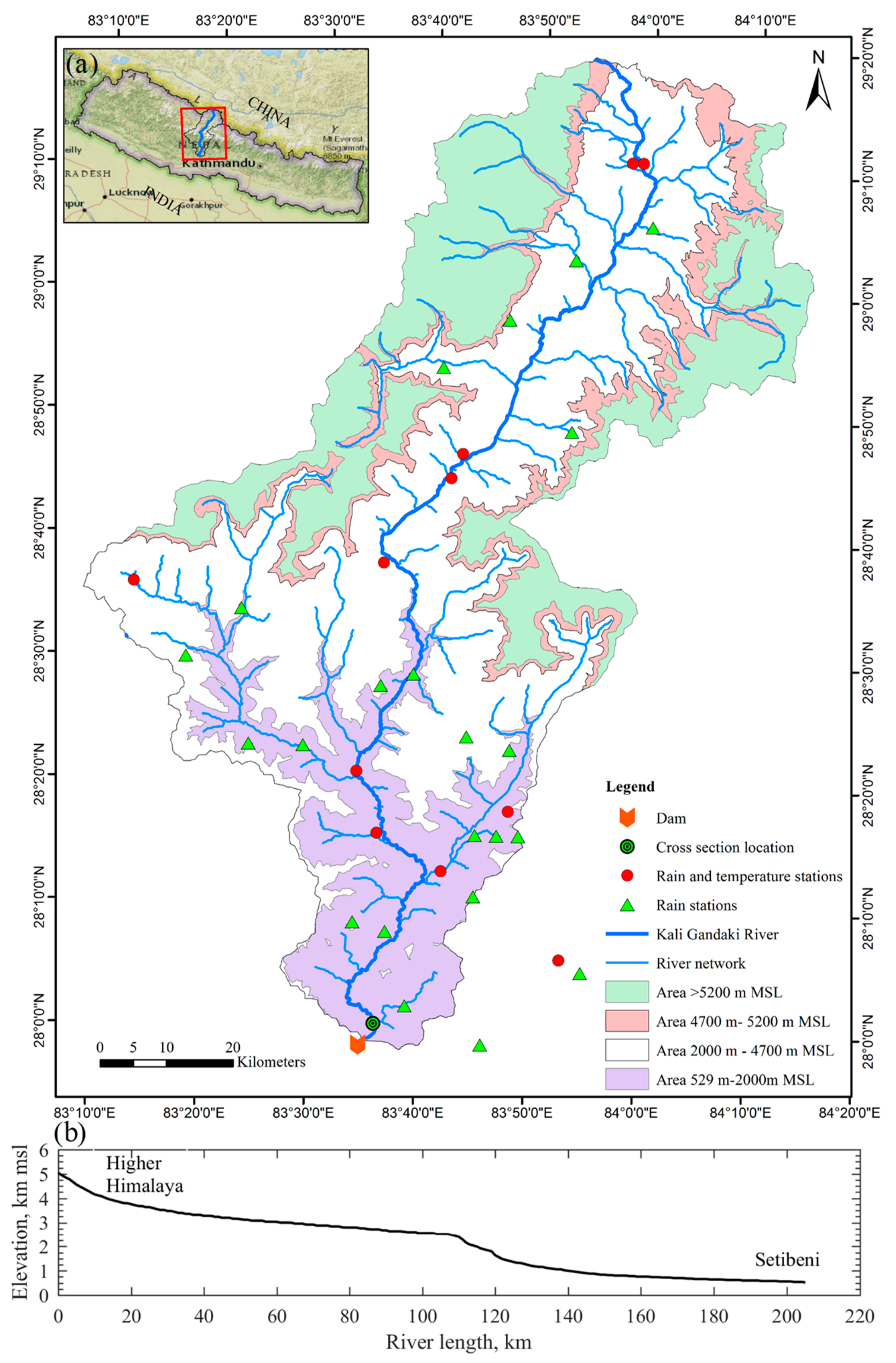
2.1. Study Site Description

The Kali Gandaki River is a glacier-fed river originating from the Himalaya region, Nepal [27]. The basin has a complex geomorphology and watershed topography with rapid changes in elevation, ranging from about 529 m MSL to 8143 m MSL. It flows from north to south in the higher Himalayan region before flowing eastward through the lower Himalayan region, entering the Terai plains of Nepal and connecting with Narayani River, which ultimately merges with the Ganges River in India. The snowfall area is separated, with elevation ranges less than 2000 m MSL having no snow cover, 2000 to 4700 m MSL having seasonal snow, 4700 to 5200 m MSL having complete snow cover except for 1 or 2 months, and elevations greater than 5200 m MSL having permanent snow [4]. The Kali Gandaki catchment basin covers a 7060 km2 area, comprised of elevations of 529~2000 m MSL covering 1317 km2 (19% coverage); 2000~4700 m MSL covering 3388 km2 (48% coverage); 4700~5200 m MSL covering 731 km2 (10% coverage); and elevations greater than 5200 m MSL covering 1624 km2 (23% coverage). Figure 1a shows the different altitude areas’ coverage map showing river networks, with the locations of meteorological stations, created in ArcGIS 10.3.1 (ERSI Inc., Berkeley, CA, USA) software. The elevations of Kali Gandaki River decrease from 5039 m MSL in the higher Himalayas to 529 m MSL at Setibeni, 5 km upstream of the hydropower dam (Figure 1b). This encompasses a wide variation in mean rainfall, ranging from less than 500 mm year−1 in the Tibetan Plateau to about 2000 mm year−1 in the monsoon-dominated Himalayas [8].
The main physiographic characteristics of the Kali Gandaki River basin at the hydropower station are shown in Table 1.
The discharge of this river varies seasonally and is dependent on the rainfall received by its tributaries’ catchments in addition to the amount of snow melting from the Himalayas. A dam (27°58′44.88′′ N, 83°34′49.68′′ E) was constructed in 2002 for a hydropower project with a 144 MW power generation capacity, at Mirmi, Syangja.

2.2. Data Collection and Acquisition

The department of Hydrology and Meteorology (DHM), Nepal established a gauge station (28°00′30′′ N, 83°36′10′′ E) in 1964 (www.dhm.gov.np) and it operated until 1995. The gauge station was not operated during the hydropower dam construction period (1997–2002). The bed level of the dam increased yearly due to the trapping of bedload as well as a suspended sediment load by the dam, which reduced the sediment load downstream. The cross-sectional areas of different years were calculated from area–discharge regression equations obtained from historical discharge rating DHM data (1964–1995). Sedimentation lowers the reservoir capacity of the dam annually.

2.3. Analysis of Shear Stress, Specific Power, and Flow Velocity

Historical discharge and cross profile elevations data sourced from Nepal Electricity Authority (NEA), Nepal were used to calculate the bed shear stress, specific power developed, and flow velocity by using the following common equations [28,29,30]:
Bed   shear   stress ,   τ b = ρ   ×   g   ×   R   ×   i .
The mean available power supply over a unit of bed area is calculated by:
ω = Ω w t = ρ   ×   g   ×   Q   ×   i w t ,
where w t represents the width of the flow, and Ω is the available stream power supply or the time rate of the energy supply to the unit length of the stream in w.m−1 and is given by:
Ω = ρ   ×   g   ×   Q   ×   i .
The flow velocity is calculated by Manning’s formula:
v = 1 n R 2 / 3 i 1 / 2 ,
where τb is the bed shear stress (N·m−2), ρ is the density of water (1000 kg·m−3), g is the acceleration due to gravity (9.81 m·s−2), R is the hydraulic radius (m), i is the slope of the river bed (m·m−1), ω is the mean available specific stream power per unit area (w·m−2), Q is the observed discharge (m3·s−1), v is the flow velocity (m·s−1), and n is Manning’s constant. Manning’s constant, n, in a steep natural channel is calculated by the equation proposed by Jarrett [31]:
n = 0.39 S 0.38 3.28 R 0.16 .

2.4. Development of Different Models for Suspended Sediment Predictions

The daily suspended sediment load transported by the river in the catchment area is a key indicator to visualize the sediment losses from the higher Himalayas and to assess the reservoir management in hydropower projects. Different researchers have developed multiple linear regression (MLR) and nonlinear multiple regression (NMLR), sediment rating curve (SRC), and artificial neural networks (ANNs) models for the prediction of the daily suspended sediment load [32,33].

2.4.1. Multiple Linear Regression

Multiple linear regression assumes that the sediment load transported by a river is in the linear form. A dependent variable, the suspended sediment load, Q s t , depends on two independent variables, the daily average discharge of a river ( Q w t ) and the average rainfall ( R t ) of a catchment area, and the model is expressed in the form of a regression equation [32,33]:
Q s t = β 0 + β 1 Q w t + β 2 R t .
The different linear models were created by considering Q w t , a day lag discharge; Q w t 1 and R t , and a day lag rainfall, R t 1 , were the input variables and the performance of different models was also evaluated.

2.4.2. Nonlinear Multiple Regression

The suspended sediment transported by the river shows a dynamic state in a nonlinear form so that it is expressed in the form of a polynomial equation [32,33]:
Q s t = β 0 + β 1 Q w t + β 2 R t + β 11 Q w t 2 + β 22 R t 2
Different nonlinear models were also created and their performance was evaluated separately.

2.4.3. Sediment Rating Curve

SRC is expressed [34] in the form of:
Q s t = a Q w t b
where Q s t is the suspended sediment load (kg·s−1), Q w t is the daily average discharge of river, and a and b are coefficients that depend on the characteristics of a river.

2.4.4. Artificial Neural Networks

An artificial neural network is capable of solving complex nonlinear relationships between input and output parameters, which consists of three different layers known as an input, hidden, and output layer, respectively [33]. MATLAB (R2016a) software was used to develop different artificial neural networks, where the input consisted of the average daily river discharge ( Q w t ), a day lag discharge ( Q w t 1 ), and average daily rainfall R t , a day lag rainfall ( R t 1 ) , where the output consisted of the average daily suspended sediment load ( Q s t ) . Out of 2191 data sets, 70% of the data was used for training, 15% for validation, and 15% for testing in the ANNs.

2.5. Model Performance

The performance of different models was assessed in terms of the root mean square (RMSE), percent BIAS (PBIAS), RMSE-observations standard deviation ratio (RSR), coefficient of determination (R2), and Nash–Sutcliffe efficiency (NSE) [32,35,36]:
R M S E = i = 1 n Q s o , i Q s p , i 2 N .
The lower the RMSE value, the better the model’s performance:
P B I A S = i = 1 n Q s o , i Q s p , i i = 1 n Q s o , i × 100 ,
where the optimal PBIAS value is 0.0, and positive values indicate a model underestimation bias and negative values indicate a model overestimation bias:
R S R = R M S E S T D E V o   =   i = 1 n Q s o , i Q s p , i 2 i = 1 n Q s o , i Q ¯ s p , i 2 .
The optimal value for RSR is 0.0; the lower the RSR, the lower the RMSE and the better the model’s performance.
Coefficient of determination:
R 2 = i = 1 n Q s o , i Q ¯ s o , i Q s p , i Q ¯ s p , i i = 1 n Q s o , i Q ¯ s o , i 2 i = 1 n Q s p , i Q ¯ s p , i 2 2 .
The optimal value for R2 is 1.0; the higher the value of R2, the better the model’s performance:
NSE =   1 i = 1 n Q s o , i Q s p , i 2 i = 1 n Q s o , i Q ¯ s o , i 2 .
The optimal value for NSE is 1.0 and values range from −∞ to 1. Values between 0.0 and 1.0 are taken as acceptable levels of performance whereas negative values indicate that the mean observed value is a better predictor than the predicted value, which indicates an unacceptable performance. Here, Q s o , i   and   Q s p , i   are the observed and predicted suspended sediment and Q ¯ s o , i   and     Q ¯ s p , i are the average observed and average predicted suspended sediment, respectively.

3. Results and Discussion

The average discharge of Kali Gandaki River from 2003 to 2012 was 306 m3·s−1 with a minimum discharge of 40.73 m3·s−1 during winter in 2009 and a maximum discharge 2824.50 of m3·s−1 during summer in 2009. The maximum discharge showed a decreasing trend from 2003 to 2006 whereas an increasing trend from 2007 onwards was observed, as shown in Figure 2a. The yearly transported sediment load increased nearby upstream river bed level elevations of the reservoir (Figure 2b) and sediment deposited into the reservoir decreased the reservoir’s capacity. The effects of climate change in the higher Himalayas appeared in the form of uneven patterns of increasing rainfall, glacial rate erosion, and permafrost degradation, resulting in an increase in landslides and debris flows [2], which also reflects the temporal and spatial variation of the water balance components in the Kali Gandaki basin [37]. The amount and intensity of rainfall around its catchment affected the discharge rating curve [27].

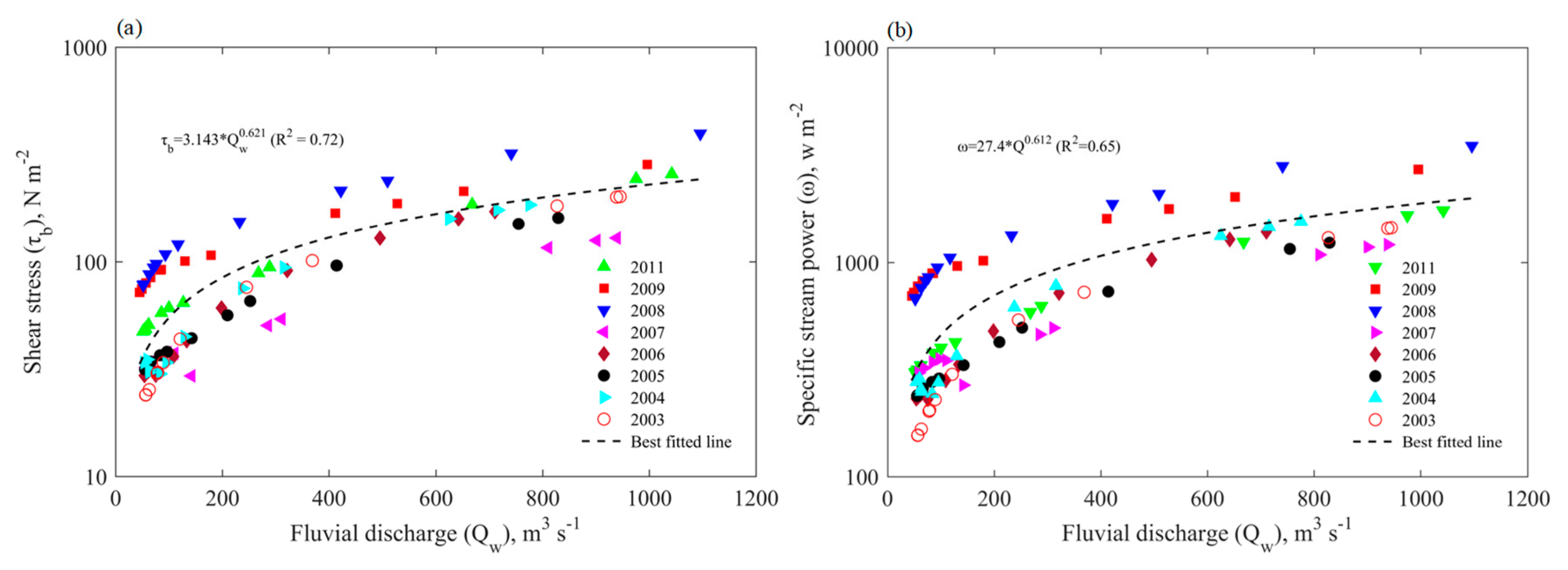
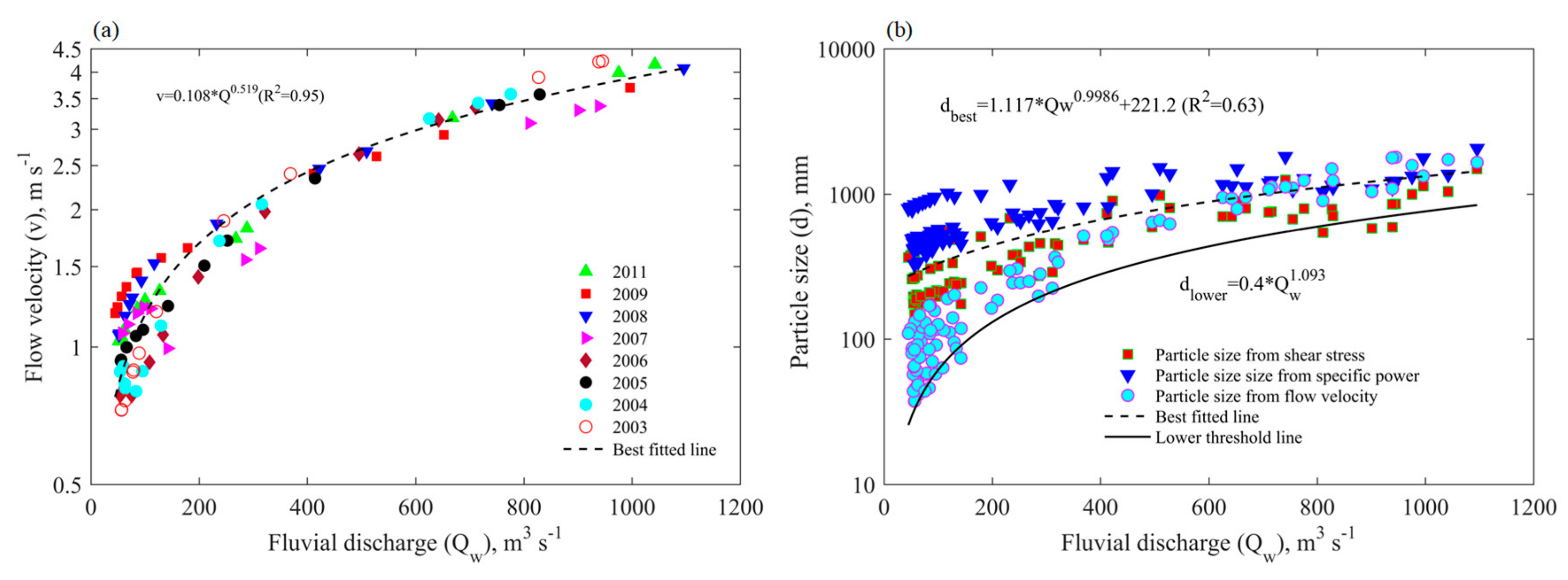
3.1. Relationship of Shear Stress, Specific Stream Power, and Flow Velocity with Discharge

The calculated shear stress, specific stream power, and flow velocity of Kali Gandaki River at the discharge gauge station, which was about 5 km upstream from the dam within limited data from 2003 to 2011, was related as:
τ b = 3.143   ×   Q 0.621   R 2 = 0.72 ,
ω = 27.40   ×   Q 0.612   R 2 = 0.65 ,
v = 0.108   ×   Q 0.519   R 2 = 0.95 .
The highest shear stress, specific stream power, and flow velocity were observed during 2008 whereas the lowest were observed during 2007. These parameters were directly related with the hydraulic radius in the case of shear stress and flow velocity, whereas the fluvial discharge in the case of specific power (Equations (1), (2), and (4)). The sedimentation process increased the bed level elevation, changing the cross geomorphology of the bed (Figure 2b). These parameters followed nearly the same trends during the remaining years. The shear stress, specific power, and flow velocity of the river increased the function of the fluvial discharge, as shown in Figure 3a,b and Figure 4a, respectively.

3.2. Relationship of Particle Sizes and Fluvial Discharge

The hydraulic parameters were the shear stress, specific stream power, and flow velocity depict transportation of different particle sizes. When subjected to the same fluvial discharge, the specific power showed an increase of 327 mm to 2062 mm particle size whereas the flow velocity depicted an increase of 37 mm to 1794 mm. The shear stress exhibited an increase of 147 mm to 1492 mm particles, which covered the lowest maximum particle sizes compared to the specific power and flow velocity (Figure 4b). These three parameters were derived from the fluvial discharge, as summarized in the lowest boundary equation form of the fluvial discharge as shown in Figure 4b:
d m m = 0.4   ×   Q 1.093   25   mm d 840   mm .
Equation (17) predicted that from the 2003 to 2011, the discharge during monsoons was capable of transporting an 840 mm particle size. Hydraulic parameters, such as the bed shear stress, specific stream power, and flow velocity, have gained wider acceptability among different researchers [20,21,22,23,24,25,26] regarding their useful contribution to the derivation of the relationship between particle sizes and hydraulic parameters. The shear stress and particle size relationship of this study was compared with Costa’s [20] average of τ b = 0.163 d 1.213 , lower boundary of τ b = 0.056 d 1.213 for 50 mm ≤ d ≤ 3290 mm; Komar’s [21] τ b = 0.164 d 1.21 for 50 mm ≤ d ≤ 5000 mm; Lenzi’s [22] τ b = 86.629 d 0.25 for 20 mm ≤ d ≤ 1000 mm; O’Connor’s [23] average of τ b = 0.0249   d 1.12 for 270 mm ≤ d ≤ 6240 mm; and Williams [24] lower boundary of τ b = 0.17 d 1.0 for 10 mm ≤ d ≤ 3300 mm (Figure 5).
For a comparative study of the specific stream power, the particle size relationship of this river was compared with Costa’s [20] average of ω = 0.030 d 1.686 and lower boundary of ω = 0.009 d 1.686 for 50 mm ≤ d ≤ 3290 mm; O’Connor’s [23] average of ω = 0.002 d 1.71 and lower boundary ω = 30 × 1.00865 d 0.1 d for a particle size of 270 mm ≤ d ≤ 6240 mm; and Williams’ [24] lower boundary of ω = 0.079 d 1.3 for a particle size of 10 mm ≤ d ≤ 1500 mm (Figure 6).
The flow velocity and particle size relationship of this study was compared with Costa’s [20] average of v = 0.20 d 0.455 and lower boundary of v = 0.14 d 0.455 for 50 mm ≤ d ≤ 3290; U.S.B.R.’s [20] v = 0.187 d 0.50 for 1 mm ≤ d ≤ 600 mm; Komar’s [21] v = 0.197 d 0.46 for 8 mm ≤ d ≤ 5000 mm; O’Connor’s [23] average of v = 0.074 d 0.60 for 270 mm ≤ d ≤ 6240 mm; Williams’ [24] lower boundary of v = 0.065 d 0.50 for 10 mm ≤ d ≤ 1500 mm; Bradely and Mears’ [25] v = 0.163 d 0.5 for 50 mm ≤ d ≤ 3290 mm; and Helley’s [26] v = 0.1545 d 0.499 for 1 mm ≤ d ≤ 600 mm (Figure 7).
The calculated values of the shear stress, specific stream power, and flow velocity were less than the observed values by Fort [6], who reconstructed the 1998 landslide dam located about 76 km upstream of the existing hydropower dam of Kali Gandaki River and estimated the hydraulic parameters with an exceptional dam breach discharge of 10,035 m3 s−1. This high discharge was responsible for the movement of a maximum boulder size of 4300 mm [6]. The higher shear stress, specific stream power, and flow velocity observed due to a higher fluvial discharge after the breaching of landslide dam were responsible for the transportation of larger sized boulders (Figure 5, Figure 6 and Figure 7).

3.3. Estimation of the Return Period by Gumbel’s Distribution

The flood return period from the historical data of DHM, Nepal can be forecasted by the Gumbel method [38] as Q T = Q ¯ + k σ n , where   Q ¯ is the mean discharge, k is the frequency factor, and σ n is the standard deviation of the maximum instantaneous flow, respectively. The frequency factor is given by k = y t y ¯ n s n , where y ¯ n is the mean and s n is the standard deviation of Gumbel’s reduced variate;   y t is given by y t = l n l n T T 1 . The observed highest flood in 1975 was 3280 m3·s−1. According to the Gumbel frequency of flood distribution, the highest flood will occur after a 40 year return period, as shown in Figure 8a, and the observed extreme discharge, as shown in Figure 8b.

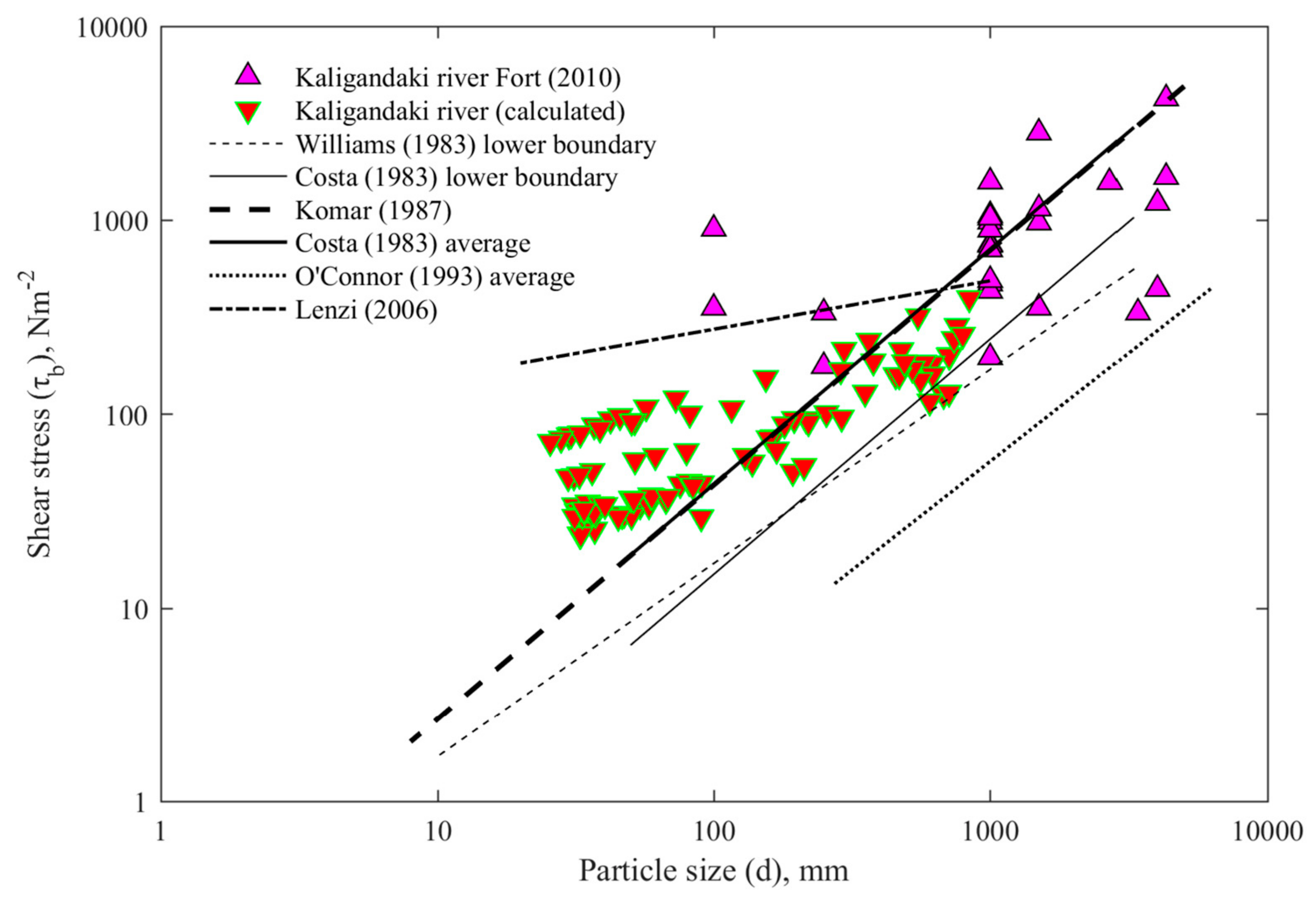
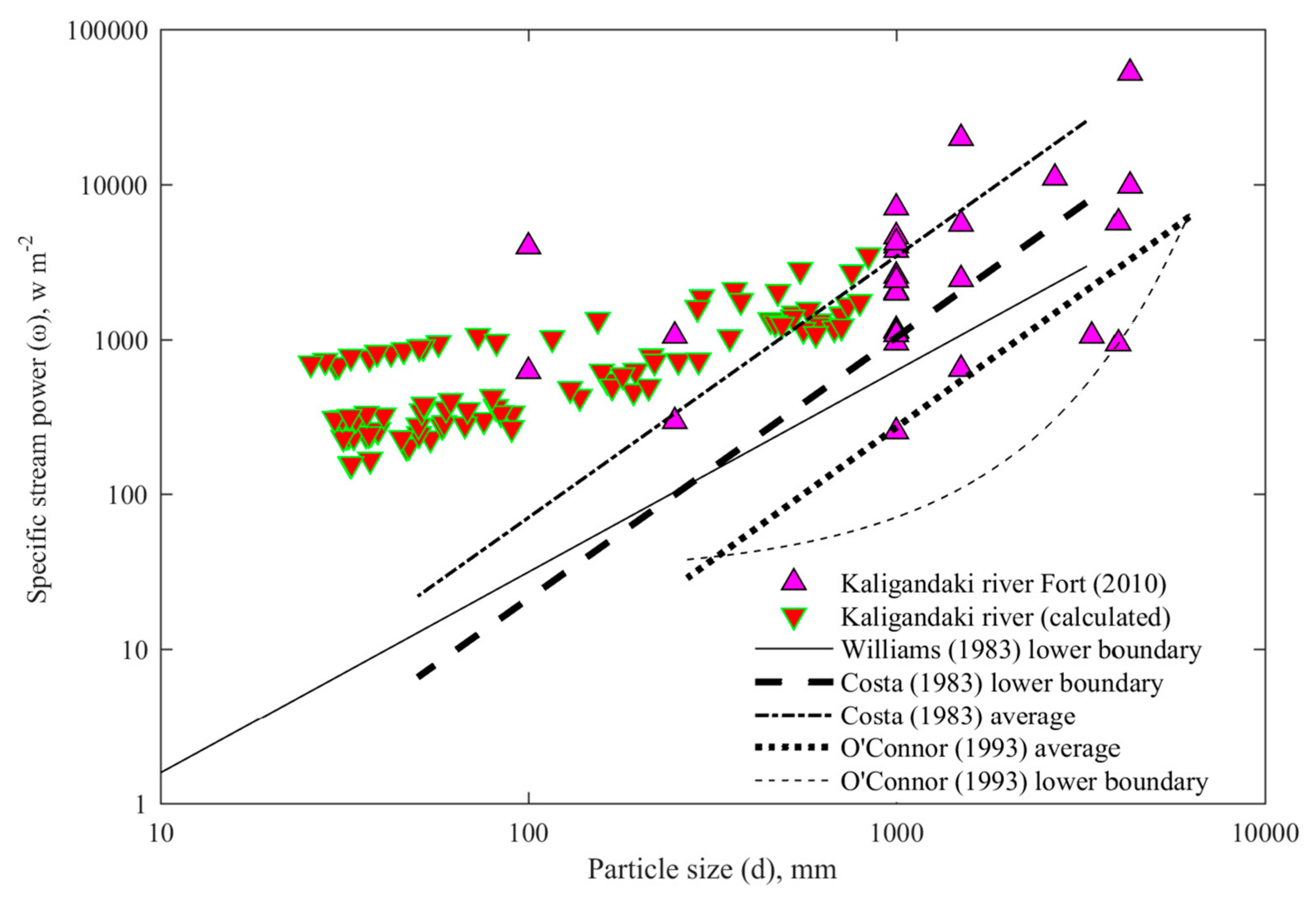
3.4. Boulder Movement Mechanisms in the Himalayas

High gradient river hydraulics are strongly influenced by large boulders, with the diameters on the same scale as the channel depth or even the width [39]. Williams [24] mentioned that five possible mechanisms of boulder transport by high gradient river are by ice, mudflow, water stepwise creep by periodic erosion, undermining of stream banks, and avalanches. The bed forming material remains immobile during typical flows, and larger bed forming particles in steep gradient channels typically become mobile only every 50 to 100 years during a hydrologic event [40]. After that, the gravel stocked in low energy sites during lower floods is mobilized and travels as the bedload [40].
The failure of the mountain slope of Kali Gandaki catchment in 1988, 1989, and 1998 was due to an evolved rock avalanche and caused the damming of the Kali Gandaki River [2]. The shockwaves after the massive 7.8 Mw Gorkha earthquake, Nepal on 25 April 2015 and its aftershocks on 23 May 2015 created cracks in the weathered rocks and weakened the mountain slopes of this catchment, which brought rocks, debris, and mud down into the river [41,42]. The river was blocked about 56 km upstream from the hydropower dam by a landslide on 24 May 2015 for 15 h [41] (Figure 9a,b). The downstream fluvial discharge after the blockage was almost zero and a flash flood occurred after an outburst of the natural landslide dam (Figure 9c,d). Extreme flooding during the monsoon period due to high rainfall and a flash flood (Figure 9b), generated by the overtopping of landslide dams [42], was responsible for the noticeable transport of large boulders in the river bed of Kali Gandaki River.
The combination of fluid stress, localized scouring, and undermining of the stream banks may cause small near vertical displacements of large boulders [43]. Catastrophic events, such as natural dam breaks and debris flows, are responsible for larger translations of boulders in rivers [40,43].

3.5. Quantification and Prediction of the Suspended Sediment

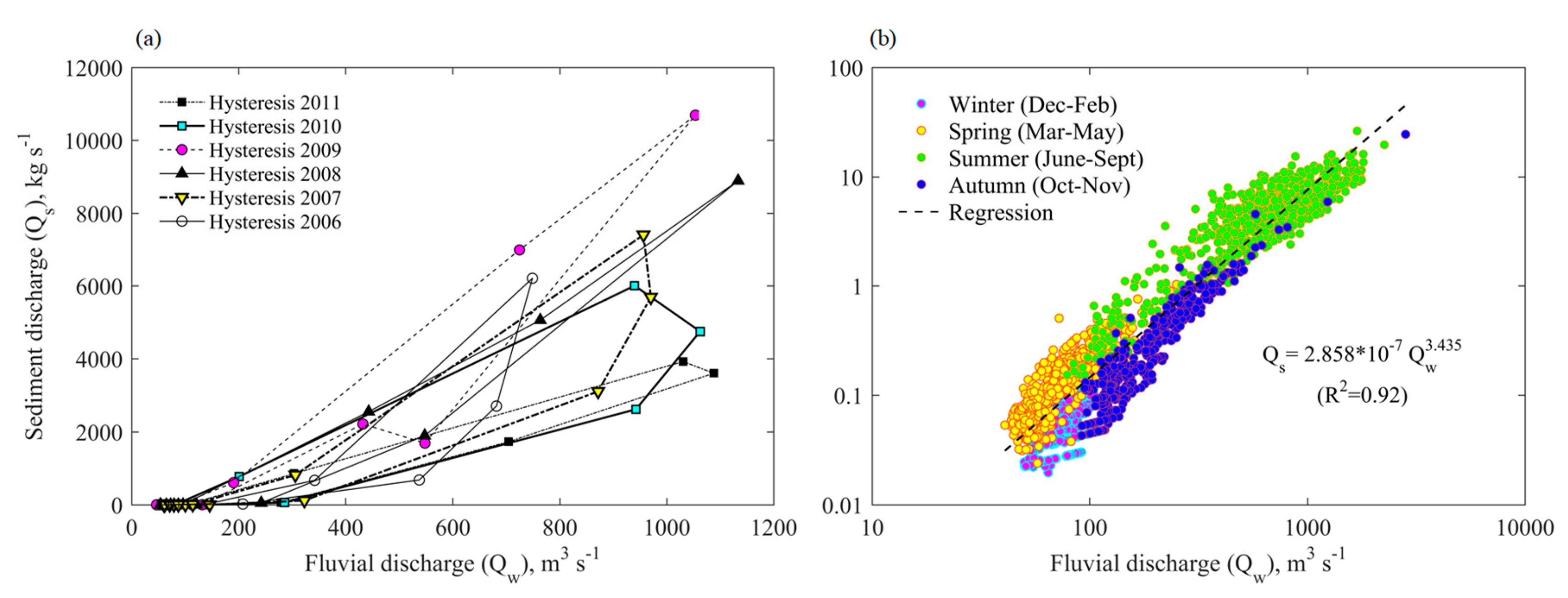
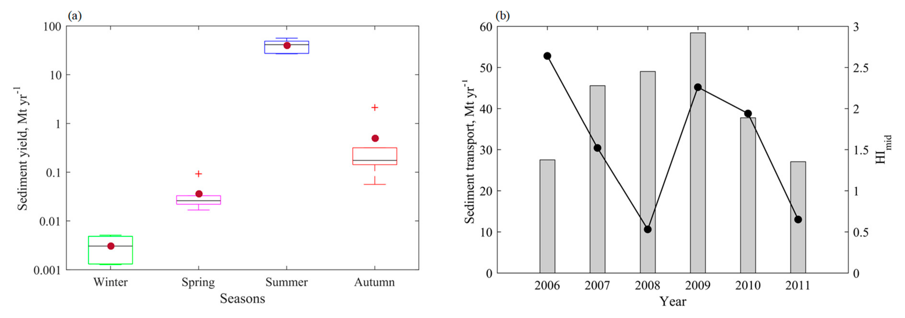
3.5.1. Hysteresis Curve and Hysteresis Index (HImid) Analysis

The relationship between the suspended sediment concentration and fluvial discharge can be studied by the nonlinear relationship between them known as hysteresis [44]. Generally, a clockwise hysteresis loop is formed due to an increasing concentration of sediment that forms more rapidly during rising limb, which suggests a source of sediment close to the monitoring point and sediment depletion in the channel system. Conversely, an anticlockwise hysteresis loop shows a long gap between the discharge and concentration peak, which suggests that the source is located far from the monitoring point or bank collapse [45,46].
Clockwise hysteresis loops were developed, increasing the suspended sediment load on the rising limb of hysteresis from December to July, leading to a maximum value of the suspended sediment load of 10,691 kg·s−1 for a fluvial discharge of 1053 m3·s−1 on August 2009. The suspended sediment load decreased on the falling limb of hysteresis from July/September to November. Overall, these six years were characterized by distinct clockwise hysteresis patterns (Figure 10a).
The HImid is a numerical indicator of hysteresis, which effectively shows the dynamic response of suspended sediment concentrations to flow changes during storm events [47].
The midpoint discharge was calculated by Lloyd [46] and Lawler [47]:
Q m i d = k Q m a x Q m i n + Q m i n ,
where k is 0.5, Q m a x is the peak discharge, and Q m i n is the starting discharge of an event.
The hysteresis index value was calculated by Lloyd [46] and Lawler [47]:
HI mid = Q s R L Q s F L 1   for   a   clockwise   loop ,
HI mid = 1 / Q s R L Q s F L + 1   for   an   anticlockwise   loop ,
where Q s R L and Q s F L are the suspended sediment on the rising and falling limb, respectively.

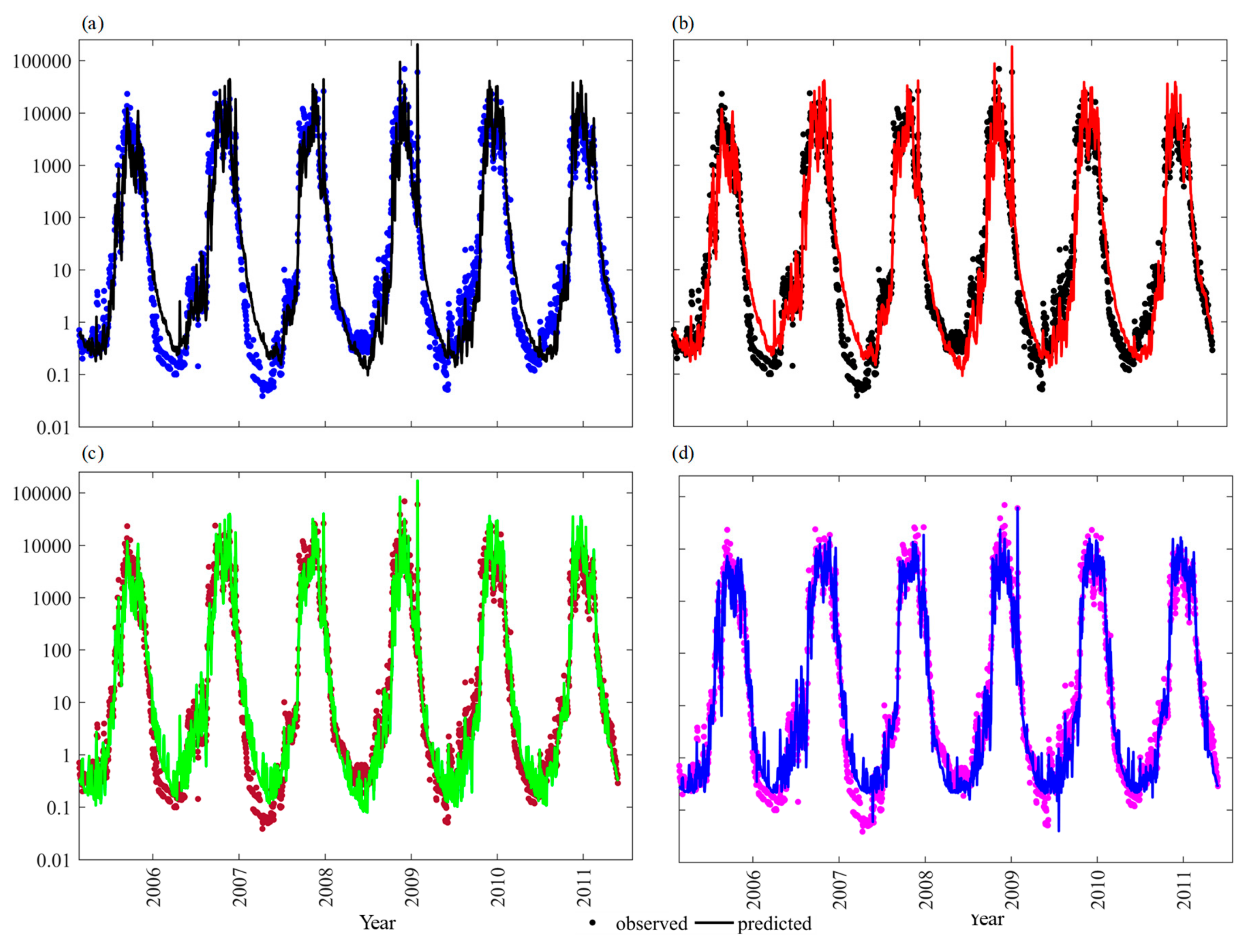
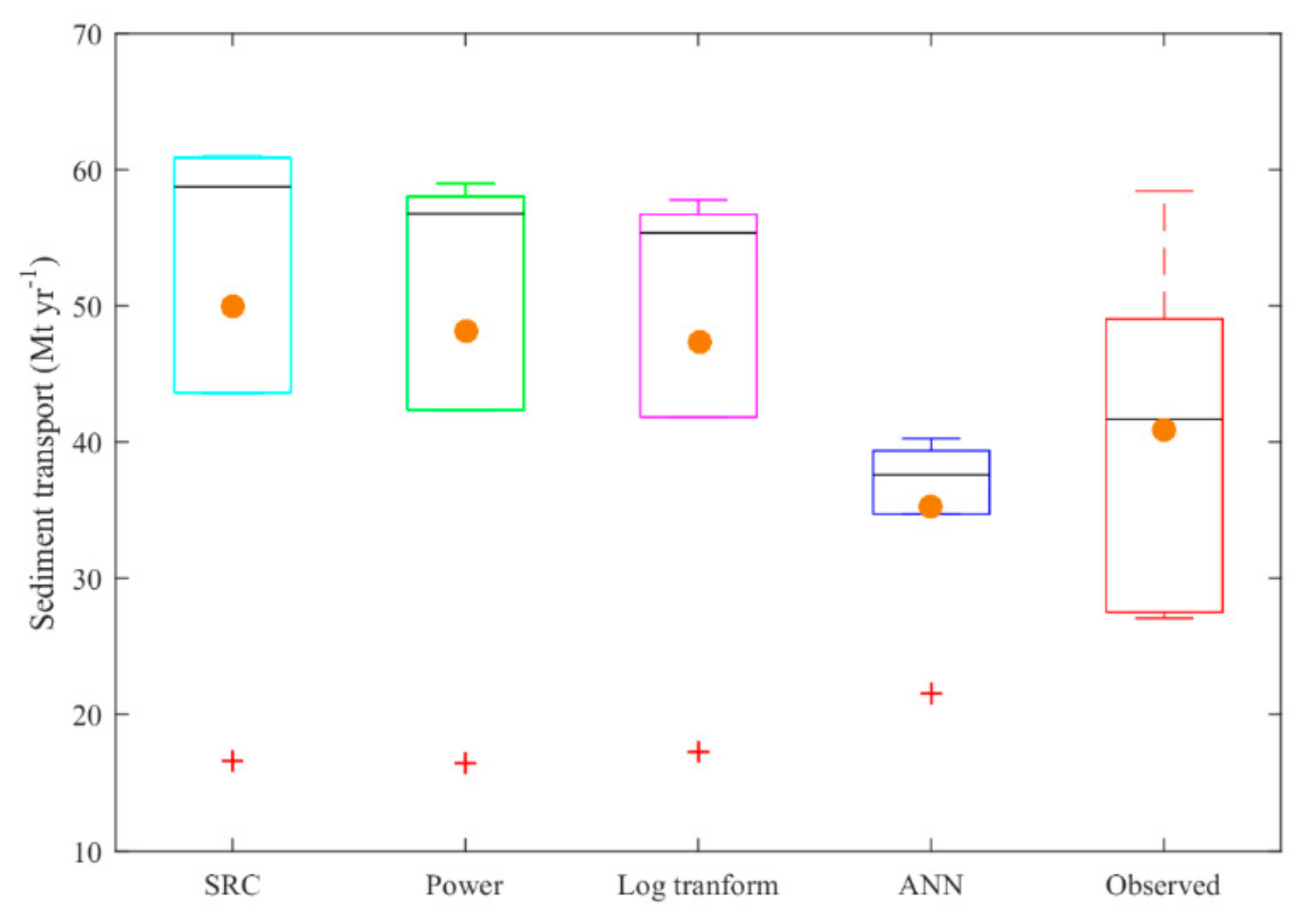
3.5.2. Yearly Suspended Sediment Yield and Prediction by Different Models

A regression equation derived from the observed data (2006 to 2011) of the suspended sediment versus the discharge of the river shown in Figure 10b is given by:
Q s = 2.858 × 10 7 × Q w 3.435 R 2 = 0.92 .
The total suspended sediment yield from the catchment is given by:
Y s = t = 0 T C w i Q w i d t = i = 1 365 C w i Q w i × 10 3 × t i + 1 t i ,
where Y s is the total annual sediment yield from the catchment,   C w i is the suspended sediment concentration in mg·L−1, Q w i is the fluvial discharge in m3·s−1,   d t is the time interval, t i and   t i + 1 are the preceding and succeeding time in seconds, respectively.
This study showed that the median ASSL transported by KaliGandaki River in the hydropower reservoir was 0.003 Mt during winter, increased to 0.026 Mt during spring, was 41.405 Mt during the summer season, and decreased 0.175 Mt during the autumn season (Figure 11a). Compared to the seasonal transport of suspended sediment, more than 96% of the suspended sediment was transported during the summer season. This depicts a wide seasonal variability of the suspended sediment caliber, which was nearly 14,000 times higher than the winter season (Figure 11a). The maximum observed ASSL transported by the river was 58.426 Mt in 2009, and after that it decreased (Figure 11b).
The HImid ≈ 0 indicated a weak hysteresis loop whereas HImid > 0 indicated a clockwise hysteresis loop, and HImid < 0 an anticlockwise hysteresis loop. Moreover, the maximum HImid developed was +2.64 in 2006, depicting the higher sediment transport rate in the rising limb but lower sediment transport rate in the falling limb (Figure 10a). The minimum HImid developed was +0.53 in 2008, depicting the nearly same paths of the rising and falling limb and indicating a weak hysteresis loop (Figure 10a and Figure 11b).
Different types of MLR, NLMR, general power, log transform linear, and ANNs models, including inputs of the fluvial discharge and average rainfall of the catchment, were developed to select the most suitable model and the results are shown in Table 2, Table 3, Table 4, Table 5 and Table 6, respectively. The performance parameters of MLR and NLMR were satisfactory but predicted negative sediment values for low fluvial discharges and low rainfall, thus these models are unacceptable.
The RMSE, PBIAS, RSR, R2, and NSE values of the general power model, log transform models, and ANNs are shown in Table 4, Table 5 and Table 6. In general, the model simulation can be judged as “satisfactory” if NSE > 0.50, and RSR ≤ 0.70, and if the PBIAS value is ±25% for the stream flow and the PBIAS value is ±55% for the sediment [35]. In this study, the predicted values from ANNs (4−10−1−1) showed an RMSE value of 1982 kg·s−1, PBIAS value of +14.26, RSR value of 0.55, R2 value of 0.71, and an NSE value of +0.70, which indicates that the ANNs model’s performance was satisfactory. Figure 12a–d show the comparison between the model’s predicted transport rates of the suspended sediment discharge in kg·s−1 of the SRC, log transform power model, log transform linear models, and ANNs and the observed suspended sediment values respectively.
Among the SRC, power, log transform, and ANN models, the best median ASSL predicted by the ANN model was 37.611 Mt for the period of 2006 to 2011, whereas the observed median ASSL was 41.678 Mt. The mean ASSL transported by the river to the hydropower reservoir was 40.904 ± 12.453 Mt for 2006 to 2011 and the ANNs’ predicted mean value was 35.190 ± 7.018 Mt (Figure 13). Struck [8] reported that the average annual suspended sediment transported by this river was 36.9 ± 10.6 Mt.

4. Conclusions

Shear stress, specific stream power, and flow velocity are important key hydraulic parameters to describe sediment transport in river systems. The monsoon fluvial discharge and landslide dam outburst flood (LDOF) were responsible for boulder movements in Kali Gandaki River, Nepal. The lower boundary equation derived from a broad range of observed and calculated data sets estimated that a maximum particle size of 840 mm was transported by the monsoon fluvial discharge from 2003 to 2011. The ASSL transported by KaliGandaki River in the hydropower reservoir increased from winter to pre-monsoon to monsoon, respectively, and decreased in the post-monsoon period. It was estimated that 40.904 ± 12.453 Mt suspended sediment is lost annually from the higher Himalayas. Additionally, the ANN model provided satisfactory results for the prediction of the suspended sediments’ transport rate in Kali Gandaki River, where the annual predicted mean ASSL value was 35.190 ± 7.018 Mt. These parameters are important for visualizing sediment loss from the higher Himalayas to the sea and also for monitoring the dead storage volume of reservoirs for hydroelectric power generation.

Author Contributions

For the conceptualization and methodology, M.B.B. and T.A.; software, validation, formal analysis, and writing—original draft preparation, M.B.B.; writing—review and editing T.A. and S.M.D.H.J.; supervision T.A.; data curation S.K.C.

Funding

This research received no external funding.

Acknowledgments

The authors would like to give thanks to Saitama University for managing the research environment. We would also like to thank to Nepal Electricity Authority for providing fluvial and sediment data and Ministry of Energy, Water Resources and Irrigation, Department of Hydrology and Meteorology, Nepal for providing historical fluvial and climate data.

Conflicts of Interest

The authors declare no conflict of interest.

References

  1. Gudino-Elizondo, N.; Biggs, T.W.; Bingner, R.L.; Langendoen, E.J.; Kretzschmar, T.; Taguas, E.V.; Taniguchi-Quan, K.T.; Liden, D.; Yuan, Y. Modelling Runoff and Sediment Loads in a Developing Coastal Watershed of the US-Mexico Border. Water 2019, 11, 1024. [Google Scholar] [CrossRef]
  2. Fort, M. Sedimentary fluxes in Himalaya. In Source-to-Sink Fluxes in Undisturbed Cold Environments; Beylich, A.A., Dixon, J.C., Zwolinski, Z., Eds.; Cambridge University Press: Cambridge, UK, 2016; pp. 326–350. [Google Scholar]
  3. Fort, M.; Cossart, E. Erosion assessment in the middle Kali Gandaki (Nepal): A sediment budget approach. J. Nepal Geol. Soc. 2013, 46, 25–40. [Google Scholar]
  4. Mishra, B.; Babel, M.S.; Tripathi, N.K. Analysis of climatic variability and snow cover in the Kaligandaki River Basin, Himalaya, Nepal. Theor. Appl. Climatol. 2014, 116, 681–694. [Google Scholar] [CrossRef]
  5. Dahal, R.K.; Hasegawa, S. Representative rainfall thresholds for landslides in the Nepal Himalaya. Geomorphology 2008, 100, 429–443. [Google Scholar] [CrossRef]
  6. Fort, M.; Cossart, E.; Arnaud-Fassetta, G. Hillslope-channel coupling in the Nepal Himalayas and threat to man-made structures: The middle Kali Gandaki valley. Geomorphology 2010, 124, 178–199. [Google Scholar] [CrossRef]
  7. Lenzi, M.A.; D’Agostino, V.; Billi, P. Bedload transport in the instrumented catchment of the Rio Cordon: Part I: Analysis of bedload records, conditions and threshold of bedload entrainment. Catena 1999, 36, 171–190. [Google Scholar] [CrossRef]
  8. Struck, M.; Andermann, C.; Hovius, N.; Korup, O.; Turowski, J.M.; Bista, R.; Pandit, H.P.; Dahal, R.K. Monsoonal hillslope processes determine grain size-specific suspended sediment fluxes in a trans-Himalayan river. Geophys. Res. Lett. 2015, 42, 2302–2308. [Google Scholar] [CrossRef] [Green Version]
  9. Asaeda, T.; Baniya, M.B.; Rashid, M.H. Effect of floods on the growth of Phragmites japonica on the sediment bar of regulated rivers: A modelling approach. Int. J. River Basin Manag. 2011, 9, 211–220. [Google Scholar] [CrossRef]
  10. Guillén-Ludeña, S.; Manso, P.; Schleiss, A. Multidecadal Sediment Balance Modelling of a Cascade of Alpine Reservoirs and Perspectives Based on Climate Warming. Water 2018, 10, 1759. [Google Scholar] [CrossRef]
  11. Megnounif, A.; Terfous, A.; Ouillon, S. A graphical method to study suspended sediment dynamics during flood events in the Wadi Sebdou, NW Algeria (1973–2004). J. Hydrol. 2013, 497, 24–36. [Google Scholar] [CrossRef]
  12. Fort, M. Sporadic morphogenesis in a continental subduction setting: An example from the Annapurna Range, Nepal Himalaya. Z. Geomorphol. 1987, 63, 36. [Google Scholar]
  13. Costa, J.E.; Schuster, R.L. The formation and failure of natural dams. Geol. Soc. Am. Bull. 1988, 100, 1054–1068. [Google Scholar] [CrossRef]
  14. O’Connor, J.E.; Costa, J.E. Geologic and hydrologic hazards in glacierized basins in North America resulting from 19th and 20th century global warming. Nat. Hazards 1993, 8, 121–140. [Google Scholar] [CrossRef]
  15. Zhang, G.; Liu, Y.; Han, Y.; Zhang, X.C. Sediment Transport and Soil Detachment on Steep Slopes: I. Transport Capacity Estimation. Soil Sci. Soc. Am. J. 2009, 73, 1291. [Google Scholar] [CrossRef]
  16. Ali, M.; Sterk, G.; Seeger, M.; Boersema, M.; Peters, P. Effect of hydraulic parameters on sediment transport capacity in overland flow over erodible beds. Hydrol. Earth Syst. Sci. 2012, 16, 591–601. [Google Scholar] [CrossRef] [Green Version]
  17. Baker, V.R.; Ritter, D.F. Competence of rivers to transport coarse bedload material. Geol. Soc. Am. Bull. 1975, 86, 975–978. [Google Scholar] [CrossRef]
  18. Lotsari, E.; Wang, Y.; Kaartinen, H.; Jaakkola, A.; Kukko, A.; Vaaja, M.; Hyyppä, H.; Hyyppä, J.; Alho, P. Geomorphology Gravel transport by ice in a subarctic river from accurate laser scanning. Geomorphology 2015, 246, 113–122. [Google Scholar] [CrossRef]
  19. Komar, P.D.; Carling, P.A. Grain sorting in gravel-bed streams and the choice of particle sizes for flow-competence evaluations. Sedimentology 1991, 38, 489–502. [Google Scholar] [CrossRef]
  20. Costa, J.E. Paleohydraulic reconstruction of flash-flood peaks from boulder deposits in the Colorado Front Range. Geol. Soc. Am. Bull. 1983, 94, 986–1004. [Google Scholar] [CrossRef]
  21. Komar, P.D. Selective Gravel Entrainment and the Empirical Evaluation of Flow Competence. Sedimentology 1987, 34, 1165–1176. [Google Scholar] [CrossRef]
  22. Lenzi, M.A.; Mao, L.; Comiti, F. When does bedload transport begin in steep boulder-bed streams? Hydrol. Process. 2006, 20, 3517–3533. [Google Scholar] [CrossRef]
  23. O’Connor, J.E. Hydrology, Hydraulics, and Geomorphology of the Bonneville Flood; Geological Society of America: Boulder, CO, USA, 1993; Volume 274, ISBN 0813722748.
  24. Williams, G.P. Paleohydrological methods and some examples from Swedish fluvial environments: I cobble and boulder deposits. Geogr. Ann. Ser. A Phys. Geogr. 1983, 65, 227–243. [Google Scholar] [CrossRef]
  25. Bradley, W.C.; Mears, A.I. Calculations of flows needed to transport coarse fraction of Boulder Creek alluvium at Boulder, Colorado. Geol. Soc. Am. Bull. 1980, 91, 1057–1090. [Google Scholar] [CrossRef]
  26. Helley, E.J. Field Measurement of the Initiation of Large Bed Particle Motion in Blue Creek Near Klamath, California; US Government Printing Office: Washington, DC, USA, 1969.
  27. Bhusal, J.K.; Subedi, B.P. Effect of climate change on suspended sediment load in the Himalayan basin: A case study of Upper Kaligandaki River. J. Hydrol. 2015, 54, 1–10. [Google Scholar]
  28. Kale, V.S.; Hire, P.S. Effectiveness of monsoon floods on the Tapi River, India: Role of channel geometry and hydrologic regime. Geomorphology 2004, 57, 275–291. [Google Scholar] [CrossRef]
  29. Mao, L.; Uyttendaele, G.P.; Iroumé, A.; Lenzi, M.A. Field based analysis of sediment entrainment in two high gradient streams located in Alpine and Andine environments. Geomorphology 2008, 93, 368–383. [Google Scholar] [CrossRef]
  30. Wicher-Dysarz, J. Analysis of Shear Stress and Stream Power Spatial Distributions for Detection of Operational Problems in the Stare Miasto Reservoir. Water 2019, 11, 691. [Google Scholar] [CrossRef]
  31. Jarrett, R.D. Hydraulics of high-gradient streams. J. Hydraul. Eng. 1984, 110, 1519–1539. [Google Scholar] [CrossRef]
  32. Uca; Toriman, E.; Jaafar, O.; Maru, R.; Arfan, A.; Ahmar, A.S. Daily Suspended Sediment Discharge Prediction Using Multiple Linear Regression and Artificial Neural Network. J. Phys. Conf. Ser. 2018, 954, 012030. [Google Scholar]
  33. Ulke, A.; Tayfur, G.; Ozkul, S. Predicting suspended sediment loads and missing data for Gediz River, Turkey. J. Hydrol. Eng. 2009, 14, 954–965. [Google Scholar] [CrossRef]
  34. Glysson, G.D. Sediment-Transport Curves; Open-File Report 87-218; US Geological Survey: Reston, VA, USA, 1987.
  35. Moriasi, D.N.; Arnold, J.G.; Van Liew, M.W.; Bingner, R.L.; Harmel, R.D.; Veith, T.L. Model evaluation guidelines for systematic quantification of accuracy in watershed simulations. Trans. ASABE 2007, 50, 885–900. [Google Scholar] [CrossRef]
  36. Pandey, M.; Zakwan, M.; Sharma, P.K.; Ahmad, Z. Multiple linear regression and genetic algorithm approaches to predict temporal scour depth near circular pier in non-cohesive sediment. ISH J. Hydraul. Eng. 2018. [Google Scholar] [CrossRef]
  37. Bajracharya, A.R.; Bajracharya, S.R.; Shrestha, A.B.; Maharjan, S.B. Climate change impact assessment on the hydrological regime of the Kaligandaki Basin, Nepal. Sci. Total Environ. 2018, 625, 837–848. [Google Scholar] [CrossRef] [PubMed]
  38. Onen, F.; Bagatur, T. Prediction of Flood Frequency Factor for Gumbel Distribution Using Regression and GEP Model. Arab. J. Sci. Eng. 2017, 42, 3895–3906. [Google Scholar] [CrossRef]
  39. Grant, G.E.; Swanson, F.J.; Wolman, M.G. Pattern and origin of stepped-bed morphology in high-gradient streams, Western Cascades, Oregon. Bull. Geol. Soc. Am. 1990, 102, 340–352. [Google Scholar] [CrossRef]
  40. Montgomery, D.R.; Buffington, J.M. Channel-reach morphology in mountain drainage basins. Bull. Geol. Soc. Am. 1997, 109, 596–611. [Google Scholar] [CrossRef]
  41. Marahatta, S. Earthquake and Ramche Landslide Dam in Kali Gandaki. Post April 25, 2015. Available online: http://coramnepal.org/wp-content/uploads/2017/09/Kali-Gandaki-Landslide-Dam-Outburst-Flood.pdf (accessed on 18 May 2019).
  42. Bricker, J.D.; Schwanghart, W.; Adhikari, B.R.; Moriguchi, S.; Roeber, V.; Giri, S. Performance of Models for Flash Flood Warning and Hazard Assessment: The 2015 Kali Gandaki Landslide Dam Breach in Nepal. Mt. Res. Dev. 2017, 37, 5–15. [Google Scholar] [CrossRef] [Green Version]
  43. Griffiths, G.A. Origin and transport of large boulders in mountain streams. J. Hydrol. 1977, 16, 1–6. [Google Scholar]
  44. Williams, G.P. Sediment concentration versus water discharge during single hydrologic events in rivers. J. Hydrol. 1989, 111, 89–106. [Google Scholar] [CrossRef]
  45. Bača, P. Hysteresis effect in suspended sediment concentration in the Rybárik basin, Slovakia/Effet d’hystérèse dans la concentration des sédiments en suspension dans le bassin versant de Rybárik (Slovaquie). Hydrol. Sci. J. 2008, 53, 224–235. [Google Scholar] [CrossRef]
  46. Lloyd, C.E.M.; Freer, J.E.; Johnes, P.J.; Collins, A.L. Using hysteresis analysis of high-resolution water quality monitoring data, including uncertainty, to infer controls on nutrient and sediment transfer in catchments. Sci. Total Environ. 2016, 543, 388–404. [Google Scholar] [CrossRef] [PubMed]
  47. Lawler, D.M.; Petts, G.E.; Foster, I.D.L.; Harper, S. Turbidity dynamics during spring storm events in an urban headwater river system: The Upper Tame, West Midlands, UK. Sci. Total Environ. 2006, 360, 109–126. [Google Scholar] [CrossRef] [PubMed]
Figure 1. (a) Map of Kali Gandaki River catchment area; (b) longitudinal profile of Kali Gandaki River.
Water 11 01229 g001
Figure 2. Yearly (a) discharge (NEA 200–2012) (b) cross profiles (2002–2011) of Kali Gandaki River.
Water 11 01229 g002
Figure 3. Relationship of fluvial discharge and (a) shear stress and (b) specific power.
Water 11 01229 g003
Figure 4. Relationship of the fluvial discharge, (a) flow velocity, and (b) particle size (boulder).
Water 11 01229 g004
Figure 5. Relationship of shear stress and particle size (boulder) and a comparison with different researchers.
Water 11 01229 g005
Figure 6. Relationship of the specific power and particle size (boulder) and a comparison with different researchers.
Water 11 01229 g006
Figure 7. Relationship of the flow velocity and particle size (boulder) and comparison with different researchers.
Water 11 01229 g007
Figure 8. (a) Gumbel flood return period, (b) extreme fluvial discharge.
Water 11 01229 g008
Figure 9. (a) Natural landslide dam formation on 24 May 2015 (~56 km upstream of dam), (b) lake formation after the blockage of the river, (c) downstream fluvial discharge after the blockage of the river, and (d) extreme fluvial discharge after breaching of the landslide dam on 25 May 2015 (Source: http://kathmandupost.ekantipur.com/news/2015-05-24/blocked-kali-gandaki-river-flows-again-with-photos.html).
Water 11 01229 g009
Figure 10. (a) Seasonal hysteresis loop of the sediment load. (b) Suspended sediment–discharge rating curve.
Water 11 01229 g010
Figure 11. (a) Seasonal suspended yield from the catchment. Central lines indicate the median, bottom and top edges of the box indicate the 25th and 75th percentiles respectively. The whiskers extend to the most extreme data points not considered outliers, the ‘+’ symbol represents outliers (1.5 fold interquartile range), the circle shows the mean value. (b) Yearly suspended sediment transport and hysteresis index (HImid).
Water 11 01229 g011
Figure 12. Observed and predicted sediment (a) SRC (Qw and Qs) model, (b) power model (Qw), (c) log transform linear model (Qw and Rt), and (d) ANN model.
Water 11 01229 g012
Figure 13. Comparison of different models’ predicted and observed yearly total suspended sediment transport. Central lines indicate the median, and bottom and top edges of the box indicate the 25th and 75th percentiles, respectively. The whiskers extend to the most extreme data points not considered outliers, the ‘+’ symbol represents outliers (1.5-fold interquartile range), and the circle shows the mean value.
Water 11 01229 g013
Table 1. Main characteristics of the river basin.
Parameters
Catchment area7060 km2
Length of river up to dam210 km
Mean gradient of river2.20%
Extreme discharge3280 m3 s−1 in 1975, 2824.5 m3 s−1 in 2009
Elevation ranges529 m MSL–8143 m MSL
PrecipitationTibetan plateau <500 mm year−1, monsoon dominated Himalayas~2000 mm year−1
Table 2. MLR models.
Model ScenarioRMSE (kg·s−1)PBIASRSRR2NSEModel Equation
Q t 2498+0.470.660.53+0.56 Q s = 7.12 Q t 920.70
R t 2729+0.340.730.44+0.47 Q s = 199.54 R t 229.07
Q t R t 2442+0.220.640.55+0.59 Q s = 5.31 Q t + 71.0 R t 897.03
Q t R t 1 2494+0.350.660.53+0.56 Q s = 6.68 Q t + 18.12 R t 1 920.66
Q t Q t 1 R t R t 1 2339+0.290.590.59+0.65 Q s = 13.47 Q t 8.02 Q t 1 14.02 R t + 64.44 R t 1 784.15
Table 3. NLMR models.
Model ScenarioRMSE (kg·s−1)PBIASRSRR2NSEModel Equation
Q t 2314+0.330.570.59+0.67 Q s = 5.02 × 10 3 Q t 2 + 0.71 Q t 111.61
R t 2697+0.660.710.46+0.49 Q s = 1.30 R t 2 + 138.75 R t 36.72
Q t R t 2280+0.150.560.61+0.68 Q s = 4.04 × 10 3 Q t 2 + 0.74 Q t + 0.57 R t 2 + 24.10 R t 188.70
Q t R t 1 2303+0.320.570.59+0.67 Q s = 5.14 × 10 3 Q t 2 0.17 Q t 0.024 R t 1 2 + 30.46 R t 1 93.99
Q t Q t 1 R t R t 1 2250+0.430.550.62+0.69 Q s = 3.73 × 10 3 Q t 2 8.10 × 10 4 Q t 1 2 + 4.97 Q t 3.02 Q t 1 + 8.18 × 10 2 R t 2 + 0.91 R t 1 2 + 8.27 R t + 0.28 R t 1 272.04
Table 4. General power model.
Model ScenarioRMSE (kg·s−1)PBIASRSRR2NSEModel Equation
General power model 1
Q t
2039+3.810.560.67+0.68   Q s = 1.027 × 10 3 Q t 2.238
General power model 2
Q t
2039+0.220.560.67+0.68   Q s = 0.847 × 10 3 Q t 2.263 + 71.08
Table 5. Log transform models.
Model ScenarioRMSE (kg·s−1)PBIASRSRR2NSEModel Equation
Linear model (SRC)
l o g Q t
4451−21.651.230.59−0.51 l o g Q s = 3.435 log Q t 6.544  
Q s = 2.858 × 10 7 Q t 3.435
General power model 2
l o g Q t
4039−17.501.120.59−0.25   l o g Q s = 3.915 l o g Q t 0.931 7.131
Linear model
l o g Q t l o g R t
3715−15.471.030.61−0.05 l o g Q s = 3.112 log Q t + 0.10 l o g R t 5.714
Table 6. ANN models.
Model ScenarioRMSE (kg·s−1)PBIASRSRR2NSEModel Equation
l o g R t
1 10 1 1
2768+54.070.770.45+0.41Levenberg-Marguardt
l o g Q t
1 10 1 1
2070+14.910.570.67+0.66Levenberg-Marguardt
l o g Q t l o g R t
2 10 1 1
2052+15.990.560.71+0.68Levenberg-Marguardt
l o g Q t l o g R t 1
2 10 1 1
2123+22.950.590.69+0.66Levenberg-Marguardt
l o g Q t l o g Q t 1 l o g R t l o g R t 1
4 10 1 1
1982+14.260.550.71+0.70Levenberg-Marguardt

