Automated Glacier Extraction Index by Optimization of Red/SWIR and NIR /SWIR Ratio Index for Glacier Mapping Using Landsat Imagery


1
College of Urban and Environmental Science, Northwest University, Xi’an 710127, China
2
Shaanxi Key Laboratory of Earth Surface System and Environmental Carrying Capacity, Northwest University, Xi’an 710127, China
3
Shaanxi Key Laboratory of Ecology and Environment of River Wetland, Weinan Normal University, Weinan 714099, China
*
Author to whom correspondence should be addressed.
Water 2019, 11(6), 1223; https://doi.org/10.3390/w11061223
Submission received: 9 May 2019
/
Revised: 30 May 2019
/
Accepted: 6 June 2019
/
Published: 12 June 2019
(This article belongs to the Section Hydrology)
Abstract
:Glaciers are recognized as key indicators of climate change on account of their sensitive reaction to minute climate variations. Extracting more accurate glacier boundaries from satellite data has become increasingly popular over the past decade, particularly when glacier outlines are regarded as a basis for change assessment. Automated multispectral glacier mapping methods based on Landsat imagery are more accurate, efficient and repeatable compared with previous glacier classification methods. However, some challenges still exist in regard to shadowed areas, clouds, water, and debris cover. In this study, a new index called the automated glacier extraction index (AGEI) is proposed to reduce water and shadow classification errors and improve the mapping accuracy of debris-free glaciers using Landsat imagery. Four test areas in China were selected and the performances of four commonly used methods: Maximum-likelihood supervised classification (ML), normalized difference snow and ice index (NDSI), single-band ratios Red/SWIR, and NIR/SWIR, were compared with the AGEI. Multiple thresholds identified by inspecting the shadowed glacier areas were tested to determine an optimal threshold. The confusion matrix, sub-pixel analysis, and plot-scale validation were calculated to evaluate the accuracies of glacier maps. The overall accuracies (OAs) created by AGEI were the highest compared to the four existing automatic methods. The sub-pixel analysis revealed that AGEI was the most accurate method for classifying glacier edge mixed pixels. Plot-scale validation indicated AGEI was good at separating challenging features from glaciers and matched the actual distribution of debris-free glaciers most closely. Therefore, the AGEI with an optimal threshold can be used for mapping debris-free glaciers with high accuracy, particularly in areas with shadows and water features.
1. Introduction
Mountain glaciers are a significant part of the cryosphere and constitute one of the most important factors of the global climate system [1]. Glacial changes are among the clearest signals of continuing global warming trends [2,3]. In recent decades, the increasing magnitude of climate change and human activities has led to substantial area and volume losses in mountain glaciers [4]. Mountain glaciers are extensive in arid areas of Northwestern China, and glacier advance or retreat significantly impacts local ecosystems and people’s lives [5]. As a result, monitoring glacier changes is essential for governments to understand ecological impacts. However, glaciers are commonly located in inaccessible remote high-mountain terrain, and traditional ground-based measurements infeasible for monitoring glaciers over a large area [6]. Thus, satellite observations commonly provide the only feasible technique for repeated-mapping of glaciers in an integrated and cost-effective manner [7,8,9]. Among the numerous types of remote-sensing data sets, Landsat data are widely acknowledged as highly valuable for glacier mapping due to the large swath width (185 km), medium spatial resolution (30 m), and long temporal series [10,11,12].
Over the years, delineating glacier boundaries using satellite data has become increasingly popular. Understanding the accuracy of these boundaries is especially significant when glacier outlines are intended as a basis for change assessment [13]. Numerous methods for multispectral glacier delineation have been developed and can be roughly categorized as two types: (1) Full manual on-screen digitization [14] and (2) automated and semi-automated methods. The former has high accuracy but is time-consuming, which significantly limits its reproducibility when analyzing glacier changes over long time periods. Conversely, automated and semi-automated methods are time-efficient in detecting debris-free glacier boundaries. Specific automated and semi-automated methods include: (1) Thresholding of ratio images [15,16], (2) unsupervised and (3) supervised classification [17,18], (4) the normalized difference snow index (NDSI) [19,20], and (5) principal component analysis (PCA) [21]. These five methods utilize the extremely low spectral reflectance of ice and snow in the shortwave infrared (SWIR) and the high reflectance in the visible and near infrared (VNIR) to identify glaciers [6]. The simple band ratio method has emerged as a ‘best’ (i.e., most simple, fast, accurate and robust) method, which includes the Red/SWIR ratio and the NIR/SWIR ratio [6,22]. On one hand, the Red/SWIR ratio identifies glaciers well under thin clouds and in shadow regions but tends to map most water features like glaciers, which is less common with the NIR/SWIR ratio. On the other hand, the NIR/SWIR ratio is inclined to miss regions with shadowed glaciers and may classify shadowed vegetation as glaciers [6,23,24]. In fact, the importance of correctly detecting shadowed areas increases at the point of minimum snow cover at the end of the melt season when the sun angle is lower. Therefore, band combination preference depends upon the amount of shadowed terrain and water within the image. However, both are present in almost every image.
To overcome these deficiencies in glacier-mapping, we propose an automated glacier extraction index (AGEI) that weighted averages the Red and NIR bands to improve the accuracy of debris-free glacier delineation. The objective of this study is to: (a) Improve accuracy of glacier mapping by automatically distinguishing glaciers in shadow and from adjacent proglacial lakes, (b) evaluate the accuracy of the AGEI in comparison with existing classification techniques, and (c) test the robustness of the AGEI in four study sites and compare Landsat results with Sentinel-2 data.
2. Study Area and Data
2.1. Study Areas
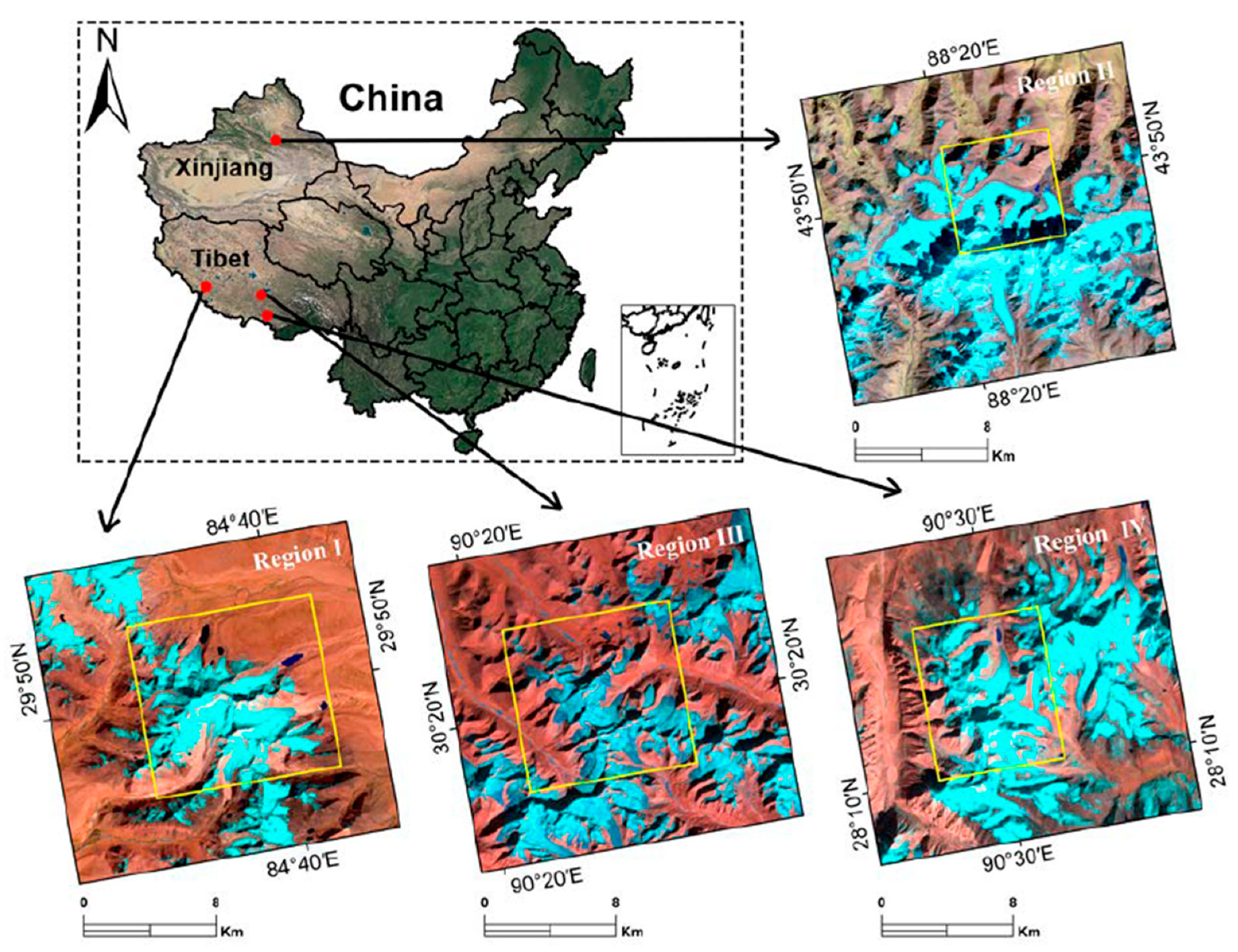
The performance and robustness of the AGEI were tested using several debris-free glaciers under different conditions in China ranging in location from Tibet to Xinjiang. Areas with challenging features including proglacial lakes and shadowed glaciers were deliberately selected as the four test sites, which are denoted as Region I, II, III, and IV (Figure 1).
Region I is in the CN5O262A0037 Gunnonggabu glacier (central longitude 84.633° E, central latitude 29.798° N), located in the Tibetan plateau, China. The glacier has a plateau semi-arid climate, the average altitude of 5848 m ranging from 5514 m to 6173 m and drains northward from mountain summits down a valley. The background of Region I includes bare land, seasonal snow, proglacial lakes, and shadowed areas. It should be noted that the Region I contains debris-covered glacier.
Region II is in the CN5Y725B0010 glacier (central longitude 88.362° E, central latitude 43.816° N), located in Xinjiang, China in a temperate continental climate. The average elevation of Region II is 3897 m, ranging from 5416 m to 3438 m. The background of Region II includes bare land, proglacial lakes, seasonal snow, and shadowed areas.
Region III is in the CN5O270C0018 Bilang Glacier (central longitude 90.407° E, central latitude 30.339° N), in a plateau semi-arid climate. The average elevation of Region III is 5890 m, ranging from 6153 m to 5660 m. The background of Region III includes bare land, proglacial lakes, and shadowed areas. In Region III, seasonal snow can be ignored.
Region IV is in the CN5O212A0165 Wujiu Glacier (central longitude 90.51° E, central latitude 28.196° N). It has a semi-arid continental climate and has an average altitude of 3897 m, ranging from 5416 m to 3438 m. The background of Region IV includes bare land, proglacial lakes, seasonal snow, and shadowed areas.
2.2. Data Sources and Pre-Processing
The first step in delineating accurate glacier boundaries from satellite data was selecting suitable images. Landsat data with no clouds and less seasonal snow was preferred, and the best scenes were collected in late summer [23]. Landsat TM and Landsat 8 images were acquired from the United States Geological Survey (USGS) website (https://glovis.usgs.gov/). All Landsat images accessed were product type L1T and had a scene quality score of nine. Sub-scenes were all free of clouds. As L1T Landsat products are geometrically corrected using the raw digital number values [24], further pre-processing (e.g., sensor calibration or topographic correction) was not needed. An atmospheric correction using the Fast Line-of-Sight Atmospheric Analysis of Spectral Hypercubes (FLAASH) module in the Environment for Visualizing Images (ENVI) 5.3 (Harris Geospatial, Broomfield, CO, United States) was used during the ML supervised classification and NDSI.
In addition to Landsat imagery, Sentinel-2 MSI data, which has a 10 m spatial resolution in visible bands and a 20 m spatial resolution in SWIR bands were also used in this study. Sentinel-2 MSI data were downloaded from the European Space Agency (ESA) website as level-1C (https://sentinel.esa.int) [25,26]. Before application of the glacier extraction index, Sentinel images were atmospherically corrected using Sen2Cor [27], which was available through the ESA’s Sentinel toolbox in the Sentinel Application Platform (SNAP).
Google Earth images, glacier inventory data, and manual glacier delineations using summer Landsat images from the same period as the experiment data were used as references for accuracy assessment. The acquisition dates of the reference data and experiment images were matched to minimize the influence of seasonal changes on the accuracy assessment. The Second Glacier Inventory Dataset of China 1.0 was provided by the “Investigation on glacier resources and their change in China” (2006FY110200) and Cold and Arid Regions Science Data Center at Lanzhou (http://westdc.westgis.ac.cn/) [28]. Glacier inventory outlines in the four test regions were extracted and showed good agreement with our manually delineated glacier boundaries. Detailed descriptions (data and date) of the satellite images and the reference data used in accuracy assessment are described in Table 1.
3. Methods
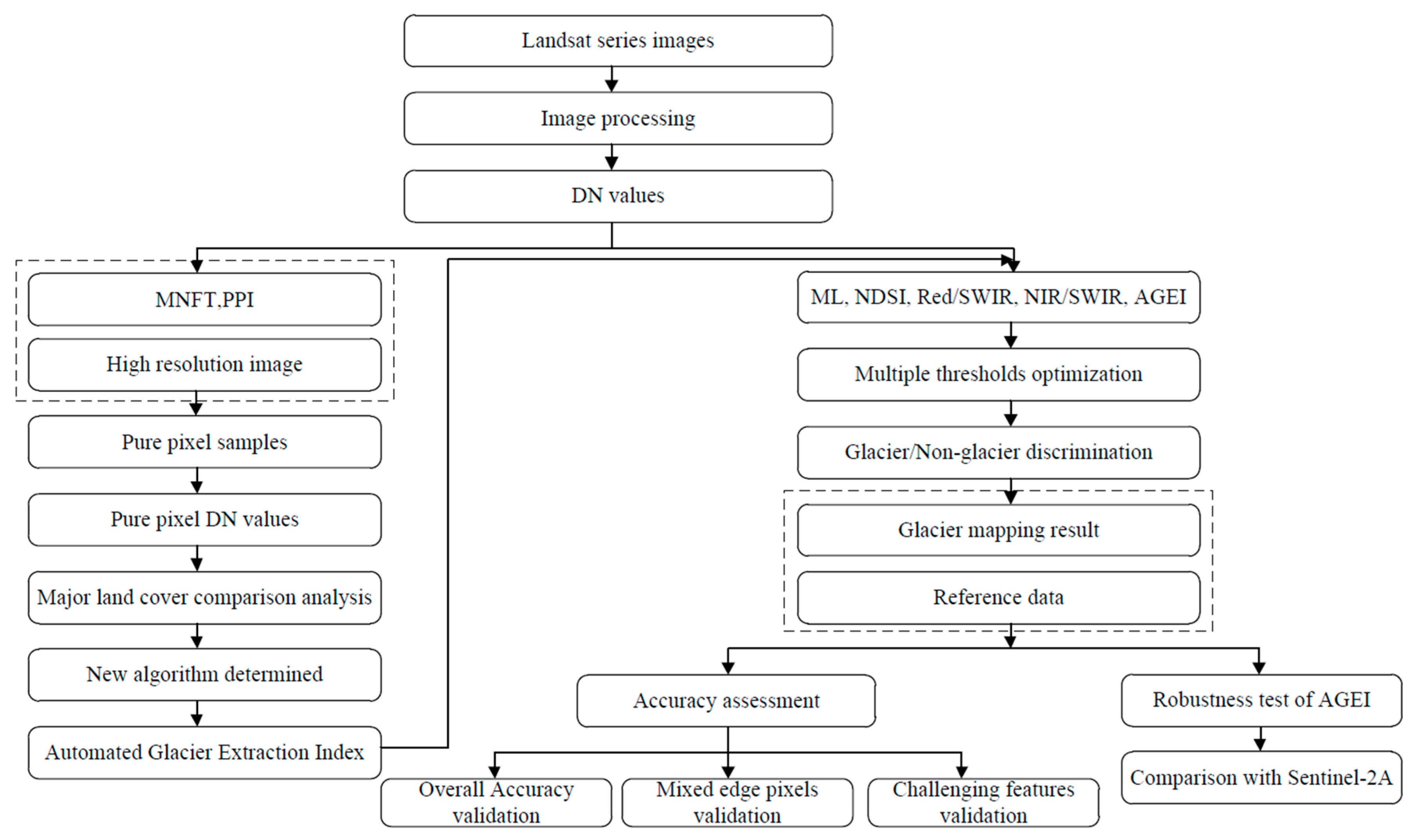
The method can be divided into six major steps: (1) Applying radiometric and atmospheric corrections to Landsat and Sentinel imagery, respectively, (2) selecting pure pixels, (3) comparing the pure pixel difference between glacier and non-glacier surfaces and developing a new index to remove water and distinguish shadowed glaciers, (4) using multiple thresholds to complete the glacier mapping, (5) assessing the accuracy of glacier extraction comprehensively using different measurements, (6) analyzing the correlation between the Landsat and Sentinel results. The specific process is shown in Figure 2.
3.1. Existing Classifiers for Glacier Mapping
Equations for calculating the four existing Landsat glacier classifiers are presented in Table 2. The supervised ML classification uses the selected region of interest (ROI) samples to define training areas for image classification. ML classification accuracy relates to sample quantity and quality. With no prior knowledge, supervised ML classification may lead to misclassifications. In addition, this approach still has limitations in glacier mapping when using multi-temporal images at large scales. Just as the normalized difference vegetation index has been widely used for mapping vegetation, NDSI is an index used to map glaciers using green band and SWIR band reflectance [29,30]. NDSI ranges from -1 to 1, and glacier features are likely to have positive values, while bare land and shadows generally have negative values. Due to the high atmospheric scattering in TM2 (green), NDSI requires more user interaction, and the path radiance has to be subtracted beforehand [31]. Thresholding of ratio images uses band ratios to maximize the difference between the target glacier and background. The Red/SWIR ratio and NIR/SWIR ratio both rely on the high reflectivity of snow and ice in the visible and near infrared and very low reflectivity in the shortwave infrared. The Red/SWIR ratio works better for shadows and thin debris-cover compared to the NIR/SWIR ratio [32]. However, the NIR/SWIR ratio is good at removing water features whose spectral reflectance is similar to glaciers. Thresholding of ratio images can be completed using raw digital number (DN) values, top-of-atmosphere (TOA) reflectance values, or spectral reflectance values [33]. Since the Red/SWIR ratio and NIR/SWIR ratio work best with raw DN values [5,6], only DN values were selected for simple band ratio calculations.
3.2. Automated Glacier Extraction Index (AGEI)
3.2.1. Pure-pixel Selection
A pure pixel is a pixel that only contains one type of land cover information, and DN values are the theoretical basis for identifying different surfaces. Pure pixels are chosen to look for cues of spectral differences between glacier and non-glacier surfaces, then provide a reference for the newly proposed index AGEI. “Pure” pixels are sampled from the Landsat 8 image of Gunnonggabu glacier, acquired on Oct. 16, 2016. This location was chosen for pure pixel extraction because Gunnonggabu includes all the major challenging features affecting glacier mapping accuracy: Debris-free glaciers, bare land, vegetation, proglacial lakes, and shadowed glaciers.
Extracting pure pixels of the selected land cover types was performed using the minimum noise fraction transform (MNFT), pixel purity index (PPI) and n-dimensional visualization. MNFT is applied to reduce noises and improve image quality. PPI is used to find the "purest" pixel in the image. Higher PPI value indicates higher pixel purity. With the help of n-dimensional visualization, the purest pixels in the data set were located, identified, and aggregated. However, not all obtained pixels were considered pure pixels. We also identified pure pixels through multi-temporal images and Google Earth images. Ultimately, pure pixel samples for glacier were taken from the glacier cap. To avoid mixed edge pixels, water/bare land pure pixel samples were taken from the middle of lakes/land. Similarly, vegetation samples were selected from a densely vegetated area. With the help of digital elevation model (DEM) and high spatial resolution aerial image from Google Earth, pure pixels of shadowed glaciers were determined.
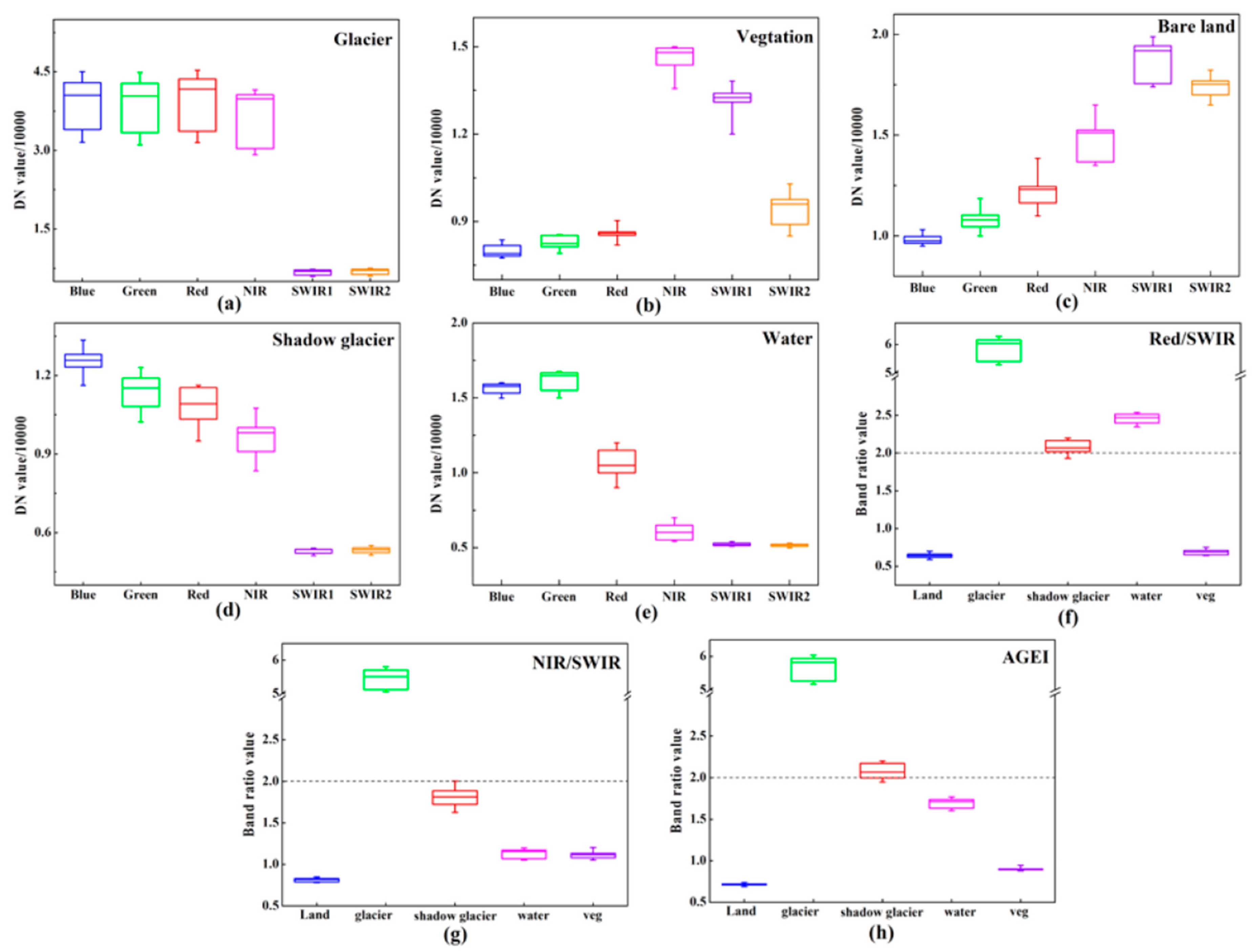
One hundred fifty-five pure pixels were extracted from the six reflective bands of the Landsat 8 image. Distributions of pure pixels DN values of major land cover types and band ratio values of different methods are shown in Figure 3. All DN values are scaled down by a factor of 10,000.
3.2.2. Formulation of AGEI
Compared to all other automatic glacier delineation techniques, the simple band ratio method with DN values emerged as a “best” (i.e., most simple, fast, accurate, and robust) [6,15,31]. Commonly used ratios include the Red/SWIR ratio and NIR/SWIR ratio. The DN value of Red band is much larger than that of the NIR band for both water feature and shadowed glacier (Figure 3d,e). However, DN values for the SWIR band for both water feature and shadowed glacier are almost the same. Therefore, Red/SWIR values for both water feature and shadow glacier are larger than NIR/SWIR values. Figure 3f,g gives the Red/SWIR and NIR/SWIR ratio for each of the five typical features using the DN. Typical threshold values are in the 2.0 ± 0.5 range for the ratio methods [6,22,32]. Both the Red/SWIR ratio and NIR/SWIR ratios can distinguish debris-free glaciers well because their ratio values are all much larger than 2.0 (the values of the glacier are distributed above the horizontal dashed line) (Figure 3f,g). The influence of bare land and vegetation can be suppressed using both ratios because ratio values are far less than 2.0 (the values of bare land and vegetation are distributed below the horizontal dashed line). For water pixels, the NIR/SWIR ratio is commonly smaller than 2.0, while the Red/SWIR ratio is larger than 2.0. For shadowed glacier pixels, the Red/SWIR ratio is mostly larger than 2.0, while the NIR/SWIR ratio is commonly smaller than 2.0. If we implement simple band ratio and use a 2.0 threshold, the Red/SWIR ratio tends to map most water surfaces as glaciers (the values of water are distributed above the horizontal dashed line) and the NIR/SWIR tends to miss shadowed glaciers (the values of shadow glacier are distributed below the horizontal dashed line). In order to reduce these errors, we propose an automated glacier extraction index (AGEI) which uses a weighted Red and NIR DN’s to substitute for the Red or NIR band. The expression of AGEI is as follows:
where α ∈ [0,1] is a weighted coefficient. An increment of 0.1 for α from 0.1 to 0.9 was set to test the AGEI algorithm. Specifically, if α=0, the AGEI is identical to the NIR/SWIR ratio, and when α = 1, the AGEI becomes the Red/SWIR ratio. Meanwhile, 2.0 can be considered an available threshold for AGEI results. When α is assigned an appropriate value, the ratio value of water pixels is smaller than 2.0 (the values of water are distributed below the horizontal dashed line), and the ratio value of shadowed glacier pixels is larger than 2.0 (the values of shadow glacier are distributed above the horizontal dashed line) (Figure 3h). Therefore, the AGEI can automatically remove water bodies from glaciers and classify shadowed glaciers as glaciers without manual correction. In this paper, four different sites were selected to test AGEI performance and four existing automated methods.
3.3. Optimization of Weighted Coefficient and Threshold
3.3.1. The Weighted Coefficient “α” of the AGEI Equation
As the main purpose of determining an optimal α is to automatically remove proglacial lakes and distinguish shadowed glaciers without manual correction, we assumed that in the Red/SWIR ratio image the value of proglacial lake pixels and shadowed glacier pixels was a1 and b1, and in the NIR/SWIR ratio image the values were assumed to be a2 and b2 respectively. The rules for selecting the optimum weighted coefficient are summarized as follows:
We know that:
In order to suppress water information and enhance shadowed glacier information, the value of water calculated from AGEI must be less than that of the shadowed glacier.
as , the optimum weighted coefficient α is in this range:
In conclusion, the optimum weighted coefficient α was between 0 and and should be adjusted within this range and determined using accuracy assessments.
3.3.2. Threshold Selection and Optimization
Multiple thresholds around 2.0 were manually chosen and tested to find the optimal threshold with the smallest total errors. Before applying a threshold to the whole scene, the optimal threshold needs to be selected after inspecting the shadowed glacier areas, which are the most sensitive to the threshold value [15,22]. The selected threshold was used to convert the ratio image into a binary glacier map. In addition, a 3 × 3 majority filter to the binary glacier map was used to remove noise [15,23].
3.4. Accuracy Validation Methods
3.4.1. Overall Accuracy Evaluation of Classified Glacier Maps
Four accuracy measures were applied, including overall accuracy, kappa coefficient, glacier total error, and non-glacier total error to evaluate the per-pixel accuracy of the classification results. The Second Glacier Inventory Dataset of China 1.0 and manual glacier delineations using summer Landsat images from the same period as the experiment data were used as references to evaluate the accuracy of classified results. The accuracy assessment procedure is summarized by the following four steps. Firstly, with multiple thresholds selected, glacier index images were classified into binary maps which only contained glacier and non-glacier areas. Next, the projection of the classified images and glacier inventory data was set to Universal Transverse Mercator (UTM)/World Geodetic System 1984 (WGS84) projection. Thirdly, glacier boundaries were manually digitized according to outlines extracted from The Second Glacier Inventory in order to evaluate the accuracy of each classified image. The above four accuracy measures were calculated based on the confusion matrix.
3.4.2. Mixed Edge Pixels Accuracy Assessment
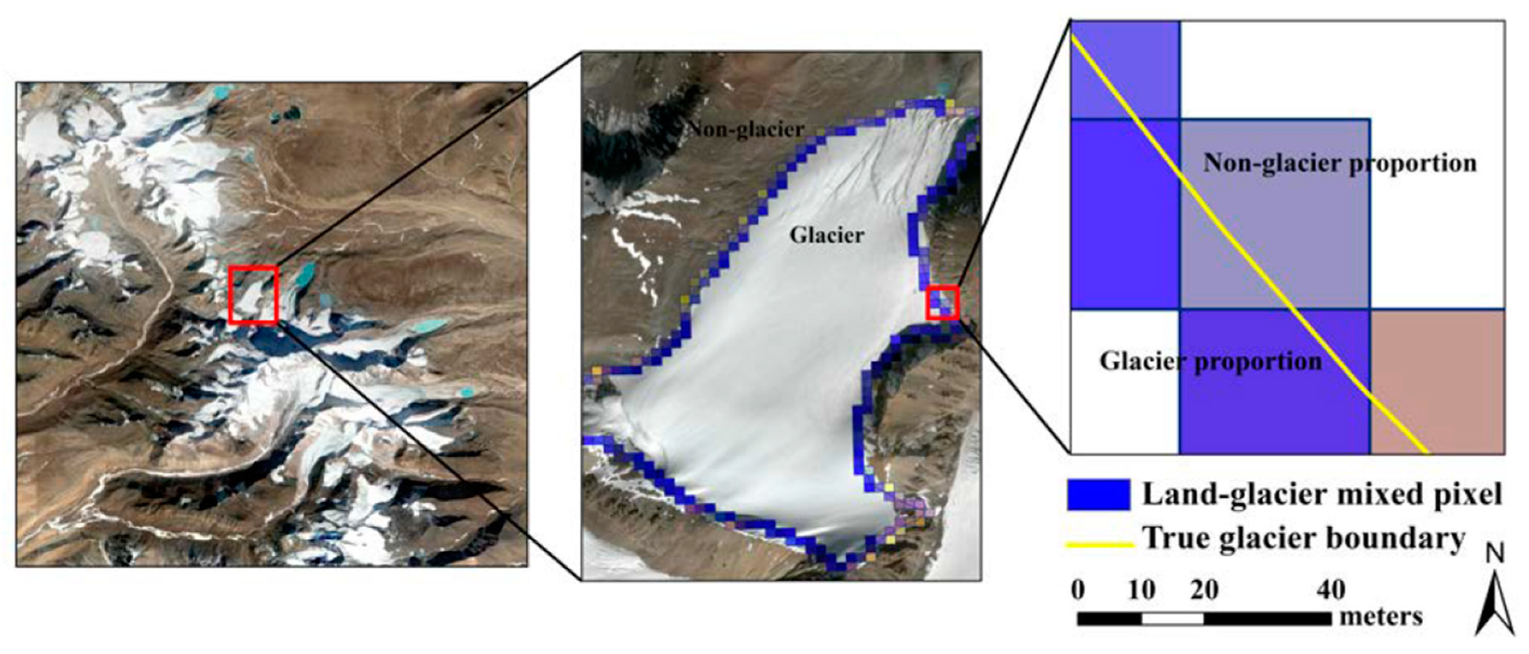
The sensitivity of AGEI and the four existing glacier extraction classifiers to various mix edge pixels of glacier and non-glacier was evaluated using sub-pixel accuracy analysis. For quantitative sub-pixel accuracy assessment, Google Earth images and an overlay analysis in ArcGIS were used [34]. Any pixel that contains both glacier and non-glacier surfaces is considered a mixed edge pixel (Figure 4). The specific validation method is as follows: (1) The Google Earth and Landsat classified images were georeferenced in the four regions, (2) “true” glacier outlines were generated by manual digitizing on the Google Earth image, (3) an overlay analysis between the “true” glacier outlines and classified glacier maps was performed, (4) the proportion of each individual mixed edge pixel covered by glacier in the four test regions was calculated, (5) graphs were drawn showing the cumulative frequency of mixed pixels classified as a glacier. It was assumed that a single mixed pixel consisting greater than 50% glacier should ideally be classified as the glacier. Conversely, when the glacier portion is less than 50% of a single pixel, the mixed pixel was considered to be non-glacier. In other words, if a mixed pixel was classified as glacier, the portion beyond the "true" boundary was considered as a commission error (over-estimation) at the sub-pixel level. Similarly, if a mixed pixel was classified as non-glacier, the fraction of it that fell inside the “true” boundary was deemed to be a sub-pixel omission error (under-estimation). A total of 2582 mixed edge pixels were selected from four test regions for sub-pixel accuracy assessment. The influence of misregistration was assumed to be insignificant.
3.4.3. Challenging Features’ Assessment at Validation Plot Scale
In order to reduce possible problems due to georeferencing of the Landsat and high-resolution data, 10 × 10 pixels validation plot samples for the TM and OLI images (300 × 300 m) were adopted for both the high-resolution images and classified glacier maps. The process of validation at plot scale is as follows: (1) The location of plot samples should be selected with challenging features: (a) Debris-free glaciers, such as glacier cap and glacier tongue, were randomly selected as plot samples, (b) challenging land features containing the debris-covered glacier and shadowed glacier were taken into consideration for plot sample selection, (c) non-glacier reference sites which are spectrally similar to glacier, including water and seasonal snow, were also added to plot samples. (2) A total of 1120 validation plot samples from four test regions were adopted for both the Google Earth images and the classified glacier maps in the locations selected in step 1. (3) Glacier area was classified by manually digitizing the shape of glaciers within each plot area using Google Earth imagery and compared with the glacier area derived from the five different classifiers, using overlay analysis and spatial connection in ArcGIS. (4) The correlation between the high-resolution glacier areas and the classified glacier areas derived from different classifiers was determined using an ordinary least squares regression.
3.5. Comparison Glacier Maps with Different Sensors
In order to test the robustness of AGEI and other four classifiers using different sensor data for glacier mapping, Landsat 8, and Sentinel-2A MSI imagery with similar acquisition times in Region I was employed [35]. We used Landsat 8 data acquired on 16 October 2016, and MSI data acquired on 23 October 2016, for the comparative analysis of Region I. It was assumed that surface conditions did not change substantially within these seven days. In this section, five classified glacier mapping results using Landsat data were overlaid with that based on Sentinel data. At the same time, the pixel percentages of the overlapped region and the non-overlapped region were calculated. The detailed results were described below.
4. Results
4.1. Comparison of Glacier Mapping Results
In this section, glacier information detected using five classifiers in four different study sites is presented. A simple visual inspection indicates that the ten classified images for the four regions all clearly show most debris-free glaciers. However, some commissions and omissions occurred (Figure 5 and Figure 6).
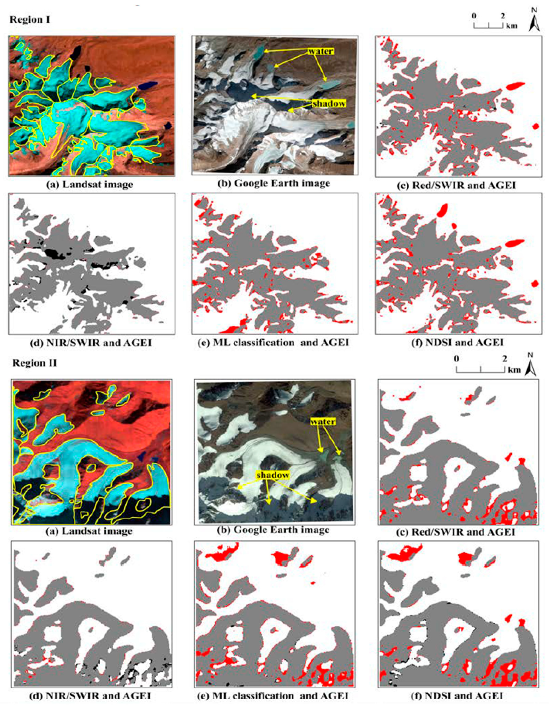
The subscenes containing hard to classify features were generally not classified correctly using automated methods. Region I contained 380 × 353 pixels, covering 120.726 km2. Major influence factors included proglacial lakes, mountainous shadows, seasonal snow, and debris-covered glaciers. For Region I, comparing the Landsat image, glacier inventory data, and Google Earth image, the NDSI and the Red/SWIR ratio produced inaccurate results (Figure 5I c,f). Numerous proglacial lake pixels were misclassified as glacier features. In contrast, the AGEI, ML supervised classification and NIR/SWIR ratio classified proglacial lakes correctly (Figure 5I d,e). By combining multitemporal images with contemporaneous high spatial resolution imagery from Google Earth, glacier inventory outlines, and Digital Elevation Model (DEM), noisy results produced by shadows were located. Although the Red/SWIR ratio, ML supervised classification, and NDSI successfully distinguished shadowed glacier, extra snowfields were also classified as glaciers (Figure 5I c,e,f). The NIR/SWIR ratio tended to ignore shadowed glaciers because the value of classified proglacial lakes and shadowed glaciers was always higher/lower than the optimal threshold (Figure 5I d). Compared with the other four classifiers, AGEI can better delineate between water and glaciers and enhance the recognition of shadowed glaciers. In areas with debris-covered glaciers, none of the five classifiers could distinguish debris because the spectral reflectance of debris was similar to surrounding rocky or sandy areas in the visible to near-infrared bands.
In Region II, there were 218 × 218 pixels, covering 42.772 km2. Shadows and snowfields were major influence factors in this site. The Red/SWIR ratio, ML supervised classification, and NDSI made a number of commission errors (Figure 5II c,e,f). Large amounts of snowfields in the shadows were classified as glaciers. Conversely, the NIR/SWIR ratio could correctly classify shadowed snowfields as non-glacier features, but some shadowed glacier pixels were neglected (Figure 5II d). The Red/SWIR ratio and NDSI also failed to exclude proglacial lakes (Figure 5II c, f). In contrast, AGEI achieved a good balance between suppressing water and enhancing shadowed glaciers.
Region III with 342 × 334 pixels covers 102.805 km2, contains proglacial lakes and shadows, and lacks snow masses. A simple visual inspection indicated that compared with AGEI, the Red/SWIR ratio and NDSI were inclined to classified non-glacier features as a glacier (Figure 6III c,f) while the NIR/SWIR ratio and ML supervised classification tended to omit shadowed glaciers (Figure 6III d,e). Region IV is 259 × 311 pixels, covers 72.4941 km2, and displays similar results to those of the first three regions. All methods other than the AGEI largely misclassified proglacial lakes and shadows (Figure 6IV c–f). None of the five classifiers could remove a large amount of seasonal snow from the image due to the similar spectral response between the glacier and seasonal snow. Therefore, suitable images with no clouds and less seasonal snow should be selected if possible.
4.2. Accuracy Assessment of Glacier Mapping
4.2.1. Overall Accuracy Evaluation of AGEI with Different Coefficients
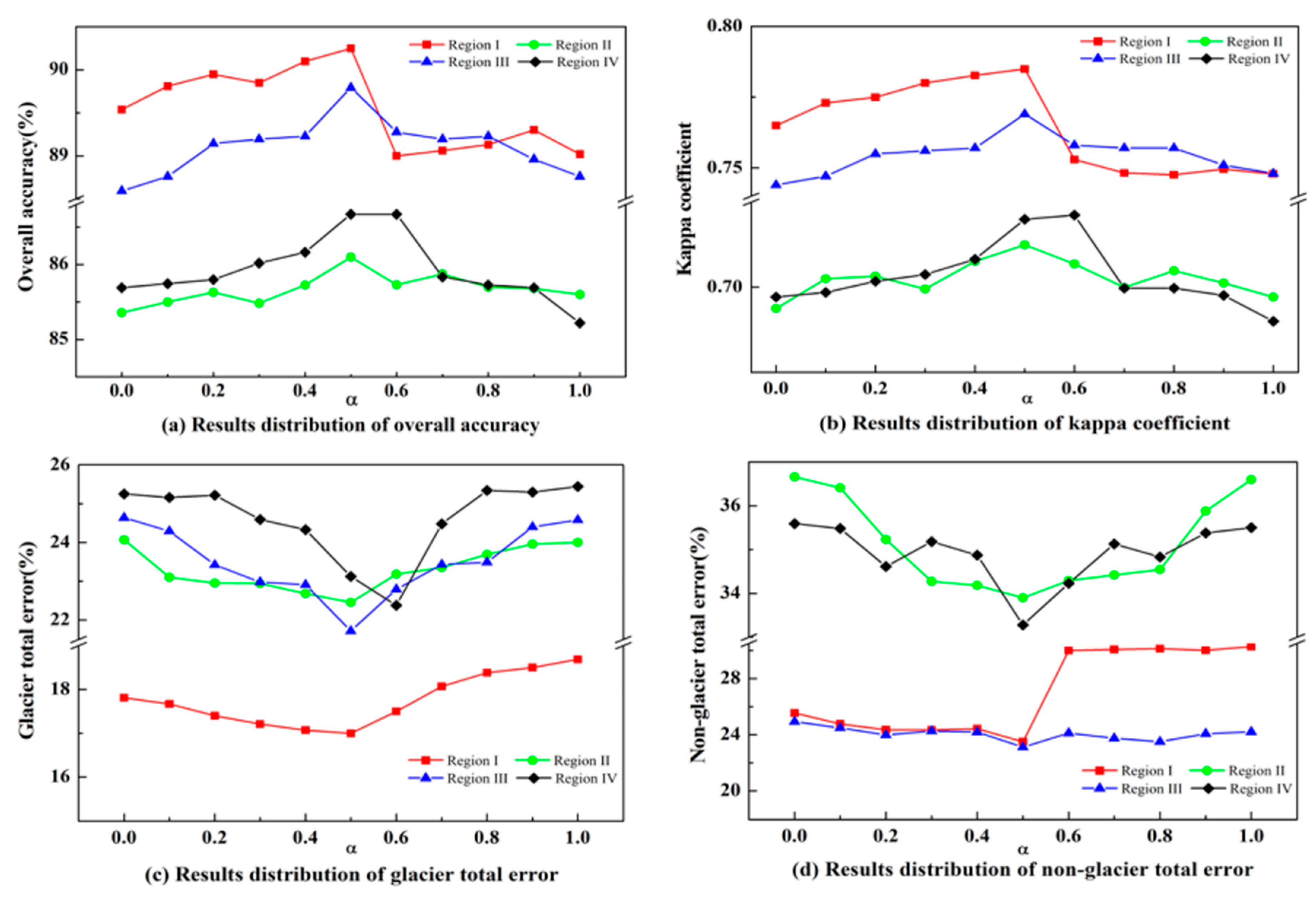
In this section, four accuracy measures: OAs, Kappa coefficients, glacier total errors, and non-glacier total errors were applied to evaluate AGEI performances with various coefficients. Glacier mapping results using AGEI with different α values were tested to find the optimal α value. An α increment of 0.1 ranging from 0.1 to 0.9 was set to obtain different AGEI outputs. Four AGEI accuracy distributions with different α values were calculated for the four test sites (Figure 7). The OA and kappa coefficient of Region I (red line) calculated using AGEI with coefficients from 0 to 0.5 were higher than those with coefficients from 0.6 to 1 (Figure 7a,b). Glacier total errors (Figure 7c) and non-glacier total errors (Figure 7d) in Region I (red line) calculated using AGEI with coefficients from 0 to 0.5 were lower than those with coefficients from 0.6 to 1. The influence of non-glacier total errors on accuracy is more significant when α is greater than 0.5 (Figure 7c,d). This was probably caused by water bodies, which primarily affect the accuracy of Region I results. On the whole, the trend line of OAs and kappa coefficients of Region I (red line) increased first and then decreased. Conversely, the trend line of glacier total errors and non-glacier total errors of Region I (red line) decreased first and then increased. Similarly, the four trend lines of the other three test regions were consistent with the trend of Region I. The peak OA and Kappa coefficient calculated by AGEI was achieved when α = 0.5 in Regions I, II, and III, as well as α = 0.5, 0.6 in Region IV (Figure 7). AGEI with α = 0.5 in Regions I, II, and III, as well as α = 0.5, 0.6 in Region IV had the lowest glacier total errors and non-glacier total errors compared with other α values. The AGEI achieved the best glacier mapping results in four test sites when α = 0.5.
4.2.2. Overall accuracy evaluation for the five classifiers with multiple thresholds
Results of mapping accuracy derived using the five classifiers in the four test sites are summarized in Table 3. The various thresholds were applied to the five classifiers images for the four test sites to obtain the highest accuracy of glacier binary maps. Numerous tests concluded that the accuracy of all investigated approaches could be partially improved by changing threshold values but at the expense of incorrect results elsewhere. Ultimately, the four appropriate thresholds for the five classifiers were determined respectively in the four regions. In the four test sites, AGEI accuracy was higher than that of the other four methods (Table 3). Quantitative assessment of Region Ⅰ showed that the maximum OA value is 90.249% (AGEI), followed by 89.54% (NIR/SWIR), 89.122% (ML supervised classification), 89.02% (Red/SWIR), and 88.094% (NDSI), respectively, and kappa coefficients is 0.785, 0.765, 0.761, 0.741, and 0.737, respectively. In Region II, the maximum OA and kappa coefficient was (AGEI) 86.10%, 0.710, followed by (Red/SWIR) 85.60%, 0.697, (NIR/SWIR) 85.359%, 0.695, (ML supervised classification) 82.336%, 0.614, and (NDSI) 79.552%, 0.540. In Region III, AGEI performed best with the highest OA 89.794% and kappa coefficients 0.769, followed by NDSI 88.96%, 0.752, Red/SWIR 88.76%, 0.748, NIR/SWIR 88.593%, 0.744, and ML supervised classification 88.024%, 0.734. Similarly, in Region IV, OA values and kappa coefficient were ranked from high to low respectively: AGEI 86.673%, 0.716, NIR/SWIR 85.691%, 0.699, Red/SWIR 85.218%, 0.692, NDSI 84.527%, 0.676, and ML supervised classification 82.691%, 0.650. Averaged over the four test sites, AGEI glacier total error, and AGEI non-glacier total error were all lower than that of NDSI, ML supervised classification, Red/SWIR ratio, and NIR/SWIR ratio.
The AGEI showed a 1%–2% accuracy improvement compared with other methods. Although this improvement seems small, the impacts of this 1%–2% improvement should not be neglected. Firstly, AGEI aims to enhance glaciers in shadowed areas and remove water bodies adjacent to glaciers. In the test region, noise factors, such as shadows and proglacial lakes, obviously account for a small proportion of subscenes. Therefore, if noise factors were inhibited, the corresponding accuracy improvement percentage would be relatively small as well. Secondly, according to data from the World Glacier Monitoring Service (WGMS) and Global Land Ice Measurements from Space (GLIMS), 0.01 km2 were identified as the optimal minimum size in glacier mapping based on Landsat and other medium-resolution remote sensing data [36,37,38]. The glacier area of the four test sites was 49.899 km2, 29.193 km2, 50.243 km2, and 55.411 km2, respectively. An accuracy improvement by 1%–2% indicates that at least 0.998 km2, 0.584 km2, 1.005 km2, and 1.108 km2 glacier areas in the four regions, respectively, were correctly classified using AGEI. Although these data cover a small area, on a large scale, ignoring them could result in a large number of glaciers being removed. By the end of 2013, the Second Glacier Inventory of China had compiled most of glaciers in western China (86%) with a total area of 43,087 km2 [39]. A 1% improvement in accuracy means that 430.87 km2 more of glacier areas would be accounted for. On a global scale, the numbers would be even larger, which has important implications for accurate water resources and climate change predictions. Thirdly, these noise factors are few but widespread. The AGEI can automatically remove proglacial lakes from glaciers and correctly classify shadowed glaciers without manual correction, minimizing the post-processing workload.
Based on the above analysis, we concluded that the AGEI outperforms the RED/SWIR ratio, NIR/SWIR ratio, NDSI, and ML supervised classification in terms of debris-free glacier mapping especially with water (proglacial lakes) and shadowed areas.
4.2.3. Mixed Edge Pixels Evaluation for the Five Classifiers
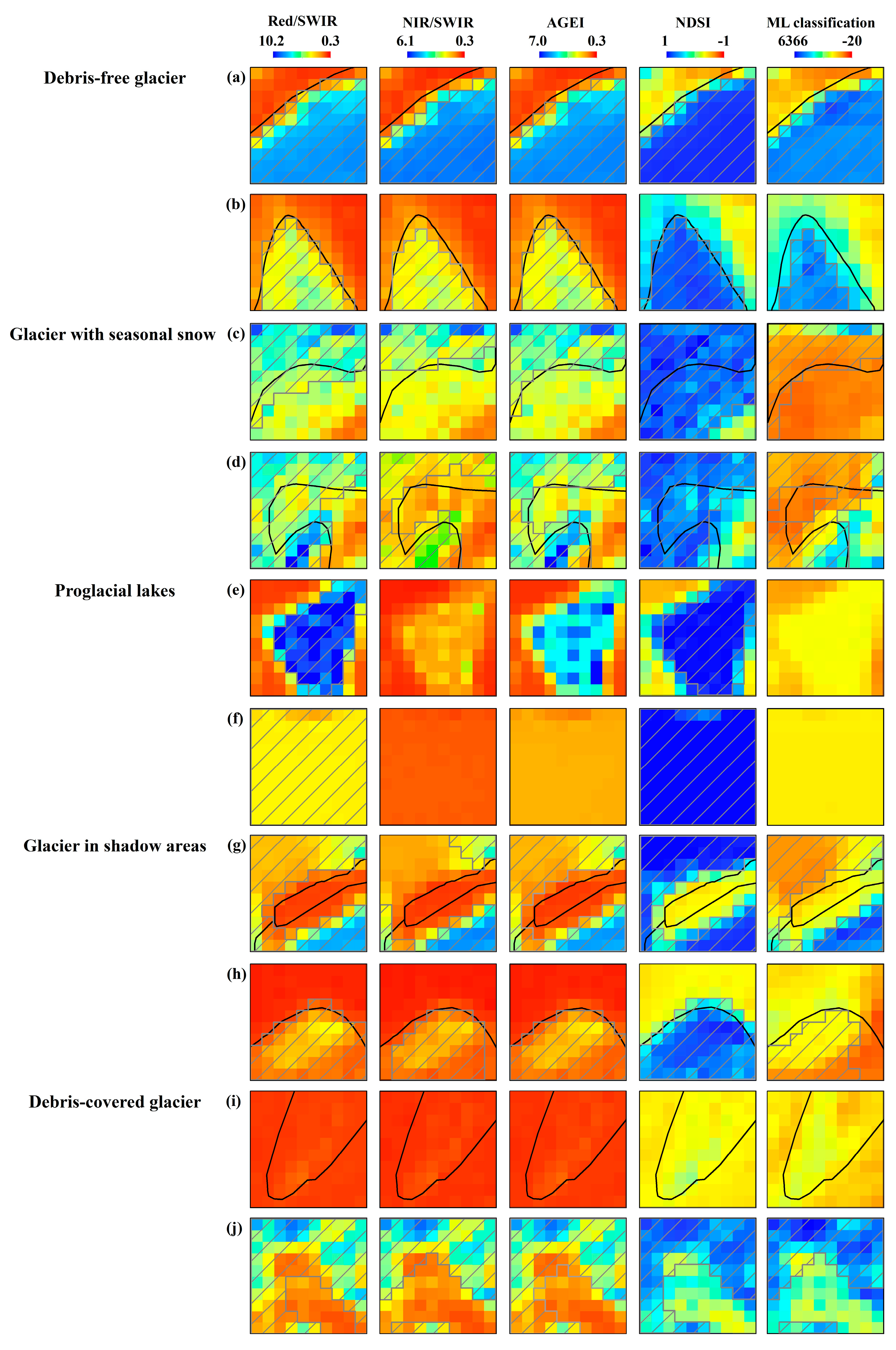
A sub-pixel accuracy assessment was performed by combing classified results with manually digitized glacier boundaries from Google Earth. The recognition ability of mixed edge pixels for the five classifiers was tested using various challenging features (Figure 8). Debris-free glacier pixels were rarely misclassified for all classifiers, with only the NIR/SWIR ratio and ML omitting a small number of edge pixels (Figure 8a,b). Glaciers with seasonal snow pixels, which had similar reflectance to glacier pixels in visible bands, had greater commission errors for the Red/SWIR ratio, NDSI, and ML (Figure 8c,d). Proglacial lake pixels, where green and red reflectance increased relative to NIR, resulted in commission errors for the Red/SWIR ratio and NDSI methods (Figure 8e,f). Omission errors increased for shadowed glacier pixels, where shadows reduced the glacier reflectance in visible bands (Figure 8g,h). All classifiers produced omission errors in edge pixels for deep shadow areas, especially the NIR/SWIR ratio (Figure 8g). The Red/SWIR ratio, and NDSI made commission errors in edge pixels and the NIR/SWIR ratio and ML lost some glacier pixels in shadowed areas (Figure 8h). Debris-covered glacier pixels, which had similar spectral reflectance to surrounding rocky or sandy areas in the visible to near-infrared wavelengths, had significant omission errors for all classifiers (Figure 8i,j).
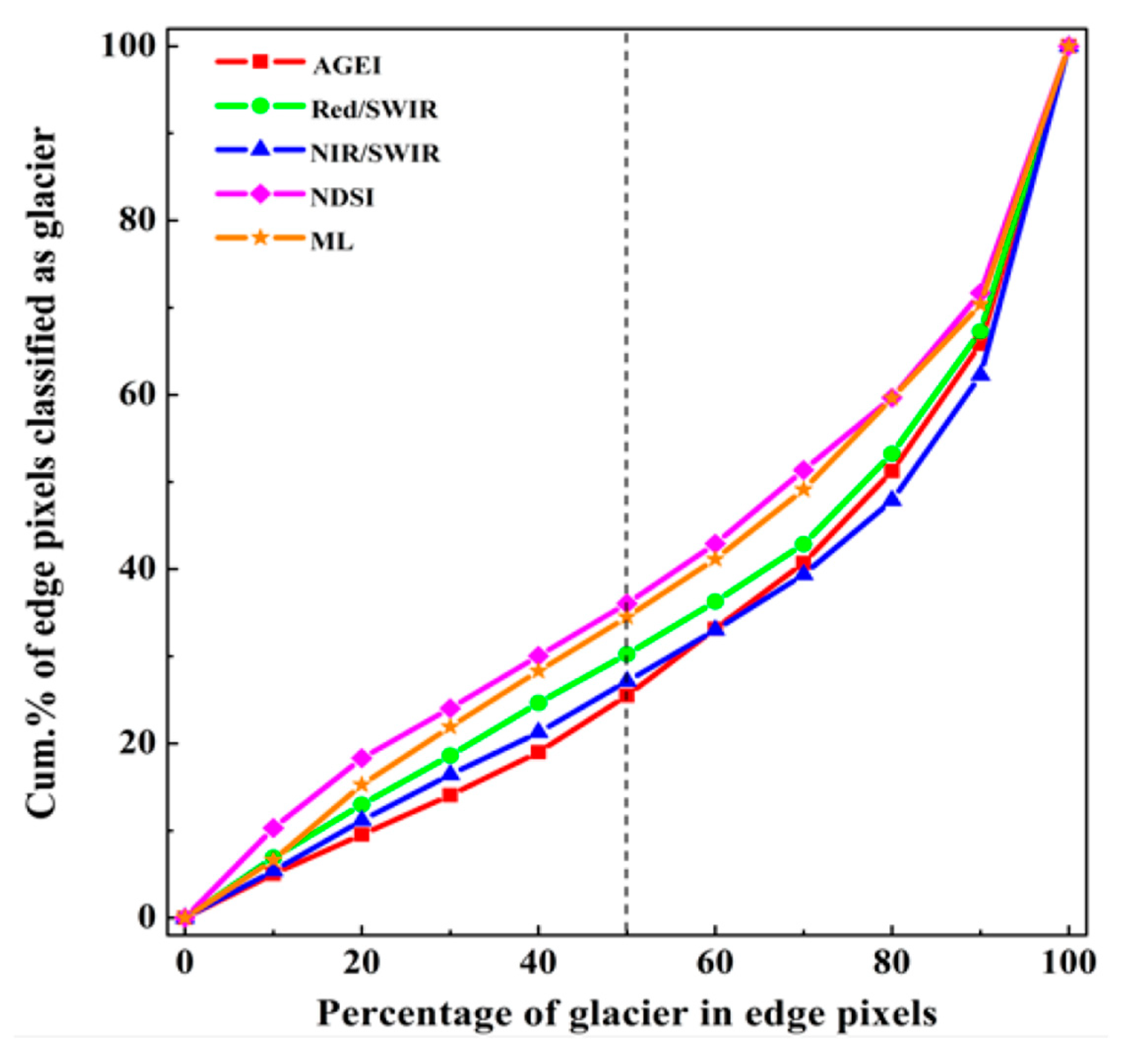
Figure 9 shows the sub-pixel accuracy analysis and cumulative frequency of mixed pixels classified as glaciers. The sensitivity of different methods to correctly recognizing edge pixels with various mixtures of the glacier and non-glacier components was compared. The vertical line in Figure 9 presents a single mixed pixel containing the 50% glacier-non glacier mixture. Edge pixels were predominantly non-glacier (<50%), and the percentage of pixels classified as glacier by the AGEI is 25.5%, which is lower than that of NIR/SWIR 27.12%, Red/SWIR 30.23%, ML supervised classification 34.51%, and NDSI 36.05%. In other words, 74.5% of mixed edge pixels classified as glacier were correctly classified by AGEI, followed by (NIR/SWIR) 72.88%, (Red/SWIR) 69.77%, (ML supervised classification) 65.49%, and (NDSI) 63.95%, respectively. According to the above results, AGEI performed better than the other four methods, and NDSI realized the lowest classification accuracy for mixed edge pixels.
4.2.4. Evaluation of Validation Plots in Different Land-Cover Backgrounds
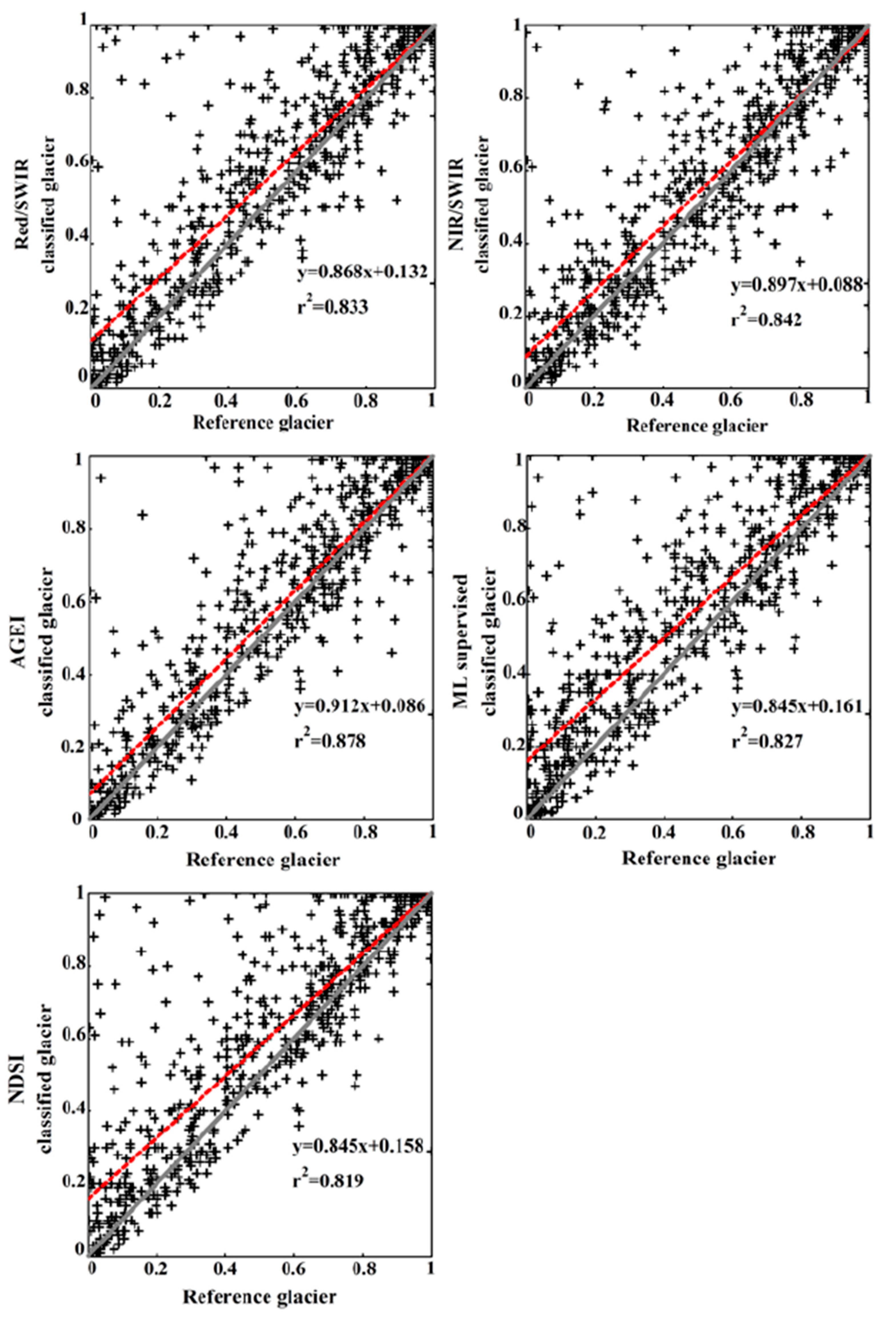
Classification accuracy at the validation plot scale (300 × 300 m) was also evaluated to compare the performance of different classifiers and minimize the influence of the geometric error between the high-resolution and Landsat images. Glacier areas from the 1120 validation plots from Google Earth images were calculated and compared with glacier areas produced by each classifier (Table 3). An ordinary least squares regression showed the correlation between the classified glacier area and the reference glacier area. For all methods, the glacier area was overestimated at the validation plot scale due to commission errors. This problem may be caused by areas with snowfields and water. Omission errors and the underestimation of glacier area were also a problem for areas with the shadowed glacier. The performance of the classifiers at the plot scale was similar to that of per-pixel assessment and sub-pixel assessment (Figure 10). The AGEI had the highest correlation (r2 = 0.878), followed by the NIR/SWIR (r2 = 0.842), Red/SWIR (r2 = 0.833), supervised ML classification (r2 = 0.827), and NDSI (r2 = 0.819) supported by slopes of 0.912, 0.897, 0.868, 0.845, and 0.845, and intercepts of 0.086, 0.088, 0.132, 0.161, and 0.158, respectively.
4.3. Comparison Glacier Mapping of Landsat and Sentinel Imagery
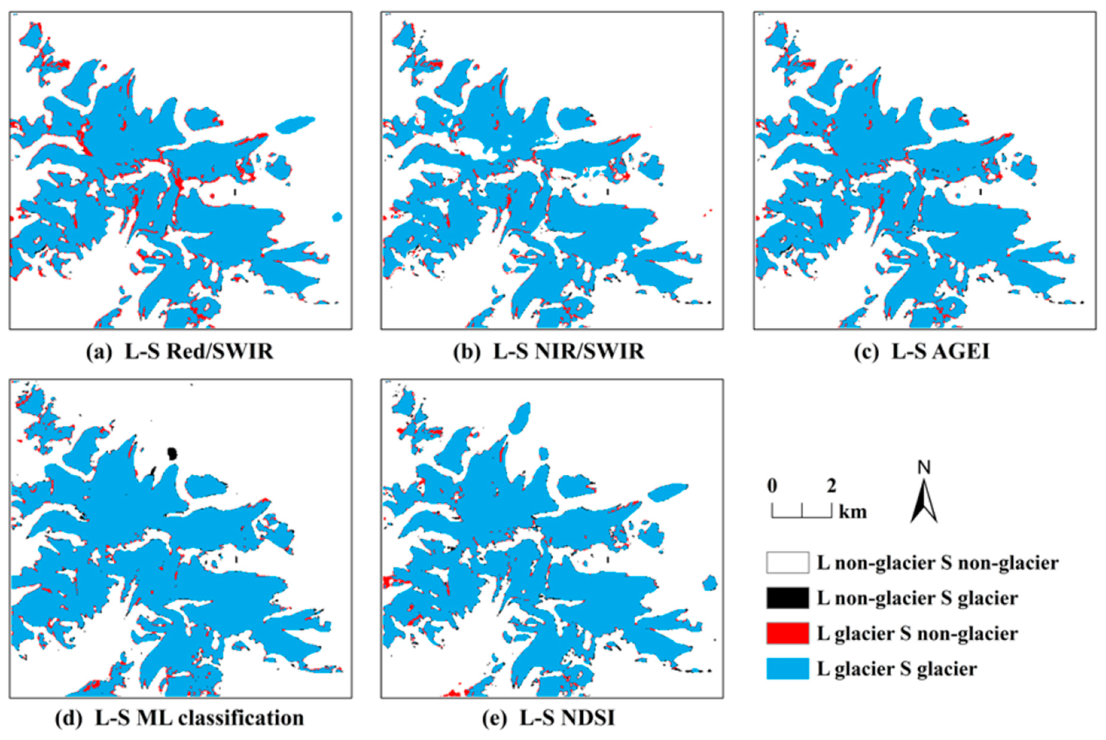
Glacier distribution maps extracted using the five methods based on Landsat and Sentinel images were overlaid and compared (Figure 11). L represented the classification results of Landsat 8 data, and S represented the classification results of Sentinel-2 data. Four pixel types were generated, which were referred to as L non-glacier S non-glacier, L glacier S glacier, L non-glacier S glacier, and L glacier S non-glacier. No matter what classifier was used, the Sentinel-2 glacial distribution was roughly consistent with the Landsat 8 distribution because all classifiers achieved high matching rate, reaching about 97% (sum of L glacier S glacier and L non-glacier S non-glacier) (Table 4). However, differences also existed in partial extraction results. Most L glacier S non-glacier pixels are located near the edge of the glacier (Figure 11 red pixels). According to the Google Earth image, Sentinel-2 data performed better than Landsat data in accurately describing glacier edges due to the higher spatial resolution. L non-glacier S glacier black pixels were mostly located in proglacial lakes, indicating Sentinel-2 data was more likely to misclassify water bodies as glaciers compared with Landsat 8 data. This may be caused by the different central wavelengths of the visible and near-infrared bands of Sentinel-2 and Landsat 8 imagery. The pixel proportion of L glacier S non-glacier was higher than that of L non-glacier S glacier, showing Sentinel-2 images obtained more non-glacier pixels using the five classifiers.
5. Discussion
The new automated glacier extraction index (AGEI) introduced in this paper can improve the accuracy of debris-free glacier mapping. Since glacier and non-glacier features have a significant spectral difference in the Red, NIR, and SWIR bands, the Red/SWIR ratio and NIR/SWIR ratio are widely used methods to delineate debris-free glaciers. However, results indicated that only using the red band (SWIR band has always been used) may tend to classify most proglacial lakes as glaciers, while only using NIR band may misclassify regions of shadowed glaciers. Since both proglacial lakes and shadows are commonly included in satellite imagery, neither the Red/SWIR ratio nor NIR/SWIR ratio can correctly classify proglacial lakes and shadowed glaciers simultaneously. In order to reduce the number of errors, the AGEI used weighted Red and NIR band values to overcome those influences and classify features correctly. From the distributions of pure pixel band ratio values, the AGEI value could be larger than that of NIR/SWIR for shadowed glaciers and smaller than that of the Red/SWIR for water features when the coefficient is properly allocated, therefore, both types of features can be classified correctly. This method uses a simple technique to distinguish shadowed glaciers and remove proglacial lakes without additional data.
Since a certain threshold value could not always achieve the highest accuracy, we explored multiple thresholds interactively selected from glaciers in shadow regions, which are the most sensitive to the threshold value. Otsu’s threshold segmentation method [40] was used for comparison. The Otsu method selects threshold values by using the rule of the maximum between-class variance of the background features and glacier features. However, experimental results using the Otsu method had low accuracy, which was far less than that of interactively selected thresholds. In addition, the selection of threshold has certain relevance with different sensors. For Landsat data, typical values of the threshold are in the 2.0±0.5 range for the AGEI and ratio methods and in the 0.4–0.9 range for the NDSI. As Sentinel data has a higher resolution than Landsat data, it can better identify the snow cover around the glacier. The optimal threshold of Sentinel data is smaller than that of Landsat data under the same image quality (the same lighting conditions, snow cover, etc.).
The weighted coefficient of AGEI can be adjusted in many scenarios to improve glacier mapping accuracy, although the adjusting process takes a long time. Experimental results from the four test regions revealed that a 0.5 coefficient achieved the highest AGEI accuracy and matched the “true” glacier boundaries most closely. However, with varying scene brightness and contrast, a certain coefficient may not always achieve the highest accuracy. Since the main purpose of determining an optimal α is to automatically classify proglacial lakes and shadowed glacier correctly, in the course of our experiment, we assumed that the value of proglacial lake pixels and shadowed glacier pixels in the Red/SWIR ratio image was a1 and b1 and in the NIR/SWIR ratio image the value was a2 and b2 respectively. Many tests lead to the conclusion that the optimum weighted coefficient α was between 0 and . When the coefficient was 0 or 1, the AGEI forms the two special cases: The NIR/SWIR ratio and Red/SWIR ratio. Therefore, the new AGEI should always perform better than or at least equal to the Red/SWIR ratio or NIR/SWIR ratio.
A comprehensive accuracy assessment for the new AGEI was carried out using three different scale validation methods: Whole-pixel, half-pixel, and plot-scale accuracy assessment. Whole pixel accuracy assessment was used to evaluate the overall accuracy (OA) of glacier classification using a confusion matrix based on full manual digitization according to glacier inventory boundaries. Half-pixel accuracy assessment was adopted to verify the sensitivity to glacier edge mixed pixels based on Google Earth images. Plot-scale validation was used to assess the ability to recognize challenging land features and serve as a complement to the half-pixel validation for eliminating the possible georeferencing errors between the Google and Landsat images. Generally speaking, for automatic glacier boundary extract methods, whole pixel accuracy evaluation results are either yes or no. Based on this, half pixel area evaluation is selected as the basis of uncertainty evaluation for edge effects [34,41]. This is particularly significant when using satellite imagery, such as Landsat, to classify land features. Due to 30 m spatial resolution of Landsat imagery, edge pixels cover relatively large areas that may be a mixture of glacier and non-glacier components. The accuracy of mixed edge pixel classification may become an important issue when using Landsat data to monitor and detect glacier changes on a global scale. With these three different accuracy validation methods, AGEI may make glacier mapping using Landsat data more accurate.
The newly proposed AGEI aims to improve the accuracy of mapping debris-free glaciers. Debris-covered glacier areas commonly have low temperature and little vegetation and are spectrally similar to surrounding rocky and sandy terrain in the visible to near-infrared wavelengths (since debris layer is derived from the valley rock materials) and are thus not mapped as a part of the glacier when only using optical images. Several studies attempted to determine a technique automatically distinguishing debris-covered glaciers [42,43,44,45]. However, all of these approaches are inefficient and are not easily applied to other test regions [6]. In the future, highly accurate automated classification methods for debris-free glacier and debris-covered glacier will likely replace manual digitization of glacier boundaries. In our test cases, AGEI was tested with Landsat and Sentinel-2 data, and it may need to be evaluated against data from other sensors. Additionally, more test sites may need to consider a thorough evaluation of AGEI performance.
6. Conclusions
In this study, we devised a new automated glacier extraction index (AGEI) to improve the accuracy of mapping debris-free glaciers, particularly in areas with proglacial lakes and shadowed glaciers that are often major causes of low classification accuracy at the end of the melt season when the sun angle is lower. The Gunnonggabu glacier, CN5Y725B0010 glacier, Bilang Glacier, and Wujiu glacier in China were selected as four test sites. Landsat imagery was used to evaluate the performance of the Red/SWIR ratio, NIR/SWIR ratio, ML supervised classification, NDSI, and AGEI. To obtain the optimal threshold for mapping glaciers, multiple thresholds were selected by inspection of shadowed glacier areas, which are most sensitive to the threshold value. During the adjustment process, the optimum weighted coefficient was assigned as 0.5 in the four test sites. Three accuracy validation methods at different scales were adopted. The per-pixel accuracy assessment indicated that the AGEI achieved the highest OAs and kappa coefficients, as well as the lowest glacier total errors and non-glacier total errors, compared with the other four methods. A sub-pixel analysis of glacier edge errors showed that the AGEI most accurately classified edge pixels. This method might be suitable for glacier change detection studies. Plot-scale validation indicated that the AGEI had the highest correlation and matched the actual glacier distribution most closely. AGEI robustness was tested for Landsat and Sentinel-2 sensors. In summary, the AGEI can be used for mapping debris-free glaciers with the highest accuracy particularly in areas with shadows and proglacial lakes.
Author Contributions
M.Z., X.W., C.S., and D.Y. jointly completed the study. The specific division of labor is as follows: methodology, M.Z. and D.Y.; software, C.S.; validation, M.Z., C.S., and X.W.; formal analysis, D.Y.; writing—original draft preparation, M.Z.; writing—review and editing, M.Z., X.W.
Funding
This study was financially supported by National Natural Science Foundation of China [Grant number 41071271], Shaanxi Province Natural Science Foundation [Grant number 2015JM4132], Strategic Priority Research Program of Chinese Academy of Sciences, China [Grant number XDA2004030201] and Shaanxi Key Laboratory of Ecology and Environment of River Wetland [Grant number SXSD201701].
Acknowledgments
Thanks to the USGS for making the Landsat archive publically available, to Cold and Arid Regions Science Data Center at Lanzhou for making The Second Glacier Inventory Dataset of China (Version 1.0) publically available, and Google for making Google Earth and the archive of imagery it displays freely available. Thanks also to the reviewers who help improve this paper significantly.
Conflicts of Interest
The authors declare no conflict of interest.
References
- Kargel, J.S. Global Land Ice Measurements from Space; Springer: Berlin/Heidelberg, Germany, 2014; pp. 205–228. [Google Scholar]
- Lemke, P.; Ren, J.; Alley, R.B.; Allison, I.; Carrasco, J.; Flato, G.; Fujii, Y.; Kaser, G.; Mote, P.; Thomas, R.H.; et al. Observations: Change in Snow, Ice and Frozen Ground; Solomon, S., Qin, D., Manning, M., Chen, Z., Marquis, M., Averyt, K.B., Tignor, M., Miller, H.L., Eds.; Cambridge University Press: Cambridge, UK, 2007; pp. 337–384. [Google Scholar]
- Stocker, T.F.; Qin, D.; Plattner, G.K.; Tignor, M.; Allen, S.K.; Boschung, J.; Nauels, A.; Xia, Y.; Bex, V. Climate Change 2013: The Physical Science Basis. Contribution of Working Group I to the Fifth Assessment Report of the Intergovernmental Panel on Climate Change; Cambridge University Press: Cambridge, UK; New York, NY, USA, 2013; p. 1535. [Google Scholar]
- Zemp, M.; Frey, H.; Gärtnerroer, I.; Nussbaumer, S.U.; Hoelzle, M.; Paul, F.; Haeberli, W.; Denzinger, F.; Ahlstrøm, A.P.; Anderson, B. Historically unprecedented global glacier decline in the early 21st century. J. Glaciol. 2015, 61, 745–762. [Google Scholar] [CrossRef] [Green Version]
- Zhang, J.; He, X.; Shangguan, D.; Zhong, F.; Liu, S. Impact of Intensive Glacier Ablation on Arid Regions of Northwest China and Its Countermeasure. J. Glaciol. Geocryol. 2012, 34, 848–854. [Google Scholar]
- Paul, F.; Bolch, T.; Kääb, A.; Nagler, T.; Nuth, C.; Scharrer, K.; Shepherd, A.; Strozzi, T.; Ticconi, F.; Bhambri, R.; et al. The glaciers climate change initiative: Methods for creating glacier area, elevation change and velocity products. Remote Sens. Environ. 2015, 162, 408–426. [Google Scholar] [Green Version]
- Immerzeel, W.W.; Kraaijenbrink, P.D.A.; Shea, J.M.; Shrestha, A.B.; Pellicciotti, F.; Bierkens, M.F.P.; de Jong, S.M. High-resolution monitoring of Himalayan glacier dynamics using unmanned aerial vehicles. Remote Sens. Environ. 2014, 150, 93–103. [Google Scholar] [CrossRef]
- Pope, A.; Rees, W.; Fox, A.; Fleming, A.H. Open access data in polar and cryospheric remote sensing. Remote Sens. 2014, 6, 6183–6220. [Google Scholar] [CrossRef]
- Pfeffer, W.T.; Arendt, A.A.; Bliss, A.; Bolch, T.; Cogley, J.G.; Gardner, A.S.; Hagen, J.; Hock, R.; Kaser, G.; Kienholz, C.; et al. The Randolph Glacier Inventory: A globally complete inventory of glaciers. J. Glaciol. 2014, 60, 537–552. [Google Scholar] [CrossRef]
- Bolch, T.; Menounos, B.; Wheate, R. Landsat-based inventory of glaciers in western Canada, 1985–2005. Remote Sens. Environ. 2010, 114, 127–137. [Google Scholar] [CrossRef]
- Rastner, P.; Bolch, T.; Mölg, N.; Machguth, H.; Le Bris, R.; Paul, F. The first complete inventory of the local glaciers and ice caps on Greenland. Cryosphere 2012, 6, 1483. [Google Scholar] [CrossRef]
- Hagg, W.; Mayer, C.; Lambrecht, A.; Kriegel, D.; Azizov, E. Glacier changes in the Big Naryn basin, Central Tian Shan. Glob. Planet. Chang. 2013, 110, 40–50. [Google Scholar] [CrossRef]
- Paul, F.; Barrand, N.E.; Baumann, S.; Berthier, E. On the accuracy of glacier outlines derived from remote-sensing data. Ann. Glaciol. 2013, 54, 171–182. [Google Scholar] [CrossRef]
- Williams, R.S.; Richard, S.; Hall, D.K.; Siguresson, O.; Chien, J. Comparison of satellite-derived with ground-based measurements of the fluctuations of the margins of Vatnajökull, Iceland, 1973–1992. Ann. Glaciol. 1997, 24, 72–80. [Google Scholar] [CrossRef]
- Paul, F.; Kääb, A.; Maisch, M.; Kellenberger, T.; Haeberli, W. The new remote-sensing-derived Swiss glacier inventory: I. Methods. Ann. Glaciol. 2002, 34, 355–361. [Google Scholar] [CrossRef] [Green Version]
- Bolch, T.; Yao, T.; Kang, S.; Buchroithner, M.; Maussion, F.; Scherer, D.; Huintjes, E.; Schneider, C. A glacier inventory for the western Nyainqentanglha Range and the Nam Co Basin, Tibet, and glacier changes 1976–2009. Cryosphere 2010, 4, 419–433. [Google Scholar] [CrossRef]
- Aniya, M.; Sato, H.; Naruse, R.; Skvarca, P.; Casassa, G. The use of satellite and airborne imagery to inventory outlet glaciers of the Southern Patagonia Icefield, South America. Photogramm. Eng. Remote Sens. 1996, 62, 1361–1369. [Google Scholar]
- Gratton, D.J.; Howarth, P.J.; Marceau, D.J. Combining DEM parameters with Landsat MSS and TM imagery in a GIS for mountain glacier characterization. IEEE Trans. Geosci. Remote Sens. 1990, 28, 766–769. [Google Scholar] [CrossRef]
- Schauwecker, S.; Rohrer, M.; Acuña, D.; Cochachin, A.; Dávila, L.; Frey, H.; Giráldez, C.; Gómez, J.; Huggel, C.; Jacques-Coper, M.; et al. Climate trends and glacier retreat in the Cordillera Blanca, Peru, revisited. Glob. Planet. Chang. 2014, 119, 85–97. [Google Scholar] [CrossRef]
- Kulkarni, A.; Patwardhan, S.; Kumar, K.K.; Ashok, K.; Krishnan, R. Projected climate change in the Hindu Kush-Himalayan region by using the high-resolution regional climate model PRECIS. Mt Res. Dev. 2013, 33, 142–151. [Google Scholar] [CrossRef]
- Sidjak, R. Glacier mapping of the Illecillewaet icefield, British Columbia, Canada, using Landsat TM and digital elevation data. Int. J. Remote Sens. 1999, 20, 273–284. [Google Scholar] [CrossRef]
- Racoviteanu, A.E.; Paul, F.; Raup, B.H.; Singh Khalsa, S.J.; Armstrong, R. Challenges and recommendations in mapping of glacier parameters from space: Results of the 2008 Global Land Ice Measurements from Space (GLIMS) workshop, Boulder, Colorado, USA. Ann. Glaciol. 2009, 50, 53–69. [Google Scholar] [CrossRef]
- Paul, F.; Bolch, T.; Briggs, K.; Kääb, A.; McMillan, M.; McNabb, R.; Nagler, T.; Nuth, C.; Rastner, P.; Strozzi, T.; et al. Error sources and guidelines for quality assessment of glacier area, elevation change, and velocity products derived from satellite data in the Glaciers_cci project. Remote Sens. Environ. 2017, 203, 256–275. [Google Scholar] [CrossRef] [Green Version]
- Landsat, N. Science Data Users Handbook; USGS: Greenbelt, MD, USA, 2018.
- Pahlevan, N.; Sarkar, S.; Franz, B.A.; Balasubramanian, S.V.; He, J. Sentinel-2 MultiSpectral Instrument (MSI) data processing for aquatic science applications: Demonstrations and validations. Remote Sens. Environ. 2017, 201, 47–56. [Google Scholar] [CrossRef]
- Veloso, A.; Mermoz, S.; Bouvet, A.; Toan, T.L.; Planells, M.; Dejoux, J.F.; Ceschia, E. Understanding the temporal behavior of crops using Sentinel-1 and Sentinel-2-like data for agricultural applications. Remote Sens. Environ. 2017, 199, 415–426. [Google Scholar] [CrossRef]
- Main-Knorn, M.; Pflug, B.; Louis, J.; Debaecker, V.; Müller-Wilm, U.; Gascon, F. Sen2Cor for Sentinel-2. In Image and Signal Processing for Remote Sensing XXIII; International Society for Optics and Photonics: Warsaw, Poland, 2017; p. 1042704. [Google Scholar]
- Guo, W.; Liu, S.; Yao, X.; Xu, J.; Shangguan, D.; Wu, L.; Zhao, J.; Liu, Q.; Jiang, Z.; Li, P.; et al. The Second Glacier Inventory Dataset of China (Version 1.0); Cold and Arid Regions Science Data Center: Lanzhou, China, 2014. [Google Scholar]
- Racoviteanu, A.E.; Arnaud, Y.; Williams, M.W.; Ordoñez, J. Decadal changes in glacier parameters in the Cordillera Blanca, Peru, derived from remote sensing. J. Glaciol. 2008, 54, 499–510. [Google Scholar] [CrossRef] [Green Version]
- Gjermundsen, E.; Mathieu, R.; Kääb, A.; Chinn, T.; Fitzharris, B.B.; Hagen, J.O. Assessment of multispectral glacier mapping methods and derivation of glacier area changes, 1978–2002, in the central Southern Alps, New Zealand, from ASTER satellite data, field survey and existing inventory data. J. Glaciol. 2011, 57, 667–683. [Google Scholar] [CrossRef]
- Paul, F.; Kääb, A. Perspectives on the production of a glacier inventory from multispectral satellite data in Arctic Canada: Cumberland Peninsula, Baffin Island. Ann. Glaciol. 2005, 42, 59–66. [Google Scholar] [CrossRef] [Green Version]
- Andreassen, L.; Paul, F. The new Landsat-derived glacier inventory for Jotunheimen, Norway, and deduced glacier changes since the 1930s. Cryosphere 2008, 2, 131–145. [Google Scholar] [CrossRef]
- Cao, M.; Li, X.; Chen, X.; Wang, J.; Che, T. Remote Sensing of Cryosphere; Science Press: Beijing, China, 2006. [Google Scholar]
- Xiong, L.; Deng, R.; Li, J.; Liu, X.; Qin, Y.; Liang, Y.; Liu, Y. Subpixel Surface Water Extraction (SSWE) Using Landsat 8 OLI Data. Water 2018, 10, 653. [Google Scholar] [CrossRef]
- Paul, F.; Winsvold, S.H.; Kääb, A.; Nagler, T.; Schwaizer, G. Glacier remote sensing using sentinel-2. Part II: Mapping glacier extents and surface facies, and comparison to Landsat 8. Remote Sens. 2016, 8, 575. [Google Scholar] [CrossRef]
- Paul, F.; Barry, R.G.; Cogley, J.G.; Frey, H.; Haeberli, W.; Ohmura, A.; Ommanney, C.S.L.; Raup, B.H.; Rivera, A.; Zemp, M. Recommendations for the compilation of glacier inventory data from digital sources. Ann. Glaciol. 2009, 50, 119–126. [Google Scholar] [CrossRef] [Green Version]
- Paul, F.; Frey, H.; Le Bris, R. A new glacier inventory for the European Alps from Landsat TM scenes of 2003, challenges and results. Ann. Glaciol. 2011, 52, 144–152. [Google Scholar] [CrossRef]
- Bliss, A.; Hock, R.; Cogley, J.G. A new inventory of mountain glaciers and ice caps for the Antarctic periphery. Ann. Glaciol. 2013, 54, 191–199. [Google Scholar] [CrossRef] [Green Version]
- Guo, W.; Liu, S.; Xu, J.; Wu, L.; Shangguan, D.; Yao, X.; Wei, J.; Bao, W.; Yu, P.; Liu, Q.; et al. The second Chinese glacier inventory: Data, methods and results. J. Glaciol. 2015, 61, 357–372. [Google Scholar] [CrossRef]
- Ohtsu, N. A Threshold Selection Method from Gray-Level Histograms. IEEE Trans. Syst. Man Cybern. 1979, 9, 62–66. [Google Scholar] [CrossRef] [Green Version]
- Xie, H.; Luo, X.; Xu, X.; Pan, H.; Tong, X. Automated subpixel surface water mapping from heterogeneous urban environments using Landsat 8 OLI imagery. Remote Sens. 2016, 8, 584. [Google Scholar] [CrossRef]
- Brenning, A.; Peña, M.A.; Long, S.; Soliman, A. Thermal remote sensing of ice-debris landforms using ASTER: An example from the Chilean Andes. Cryosphere 2012, 6, 367–382. [Google Scholar] [CrossRef]
- Bhambri, R.; Bolch, T.; Chaujar, R.K. Mapping of debris-covered glaciers in the Garhwal Himalayas using ASTER DEMs and thermal data. Int. J. Remote Sens. 2011, 32, 8095–8119. [Google Scholar] [CrossRef] [Green Version]
- Wang, L.; Chen, Y.; Tang, L.; Fan, R.; Yao, Y. Object-Based Convolutional Neural Networks for Cloud and Snow Detection in High-Resolution Multispectral Imagers. Water 2018, 10, 1666. [Google Scholar] [CrossRef]
- Rastner, P.; Bolch, T.; Notarnicola, C.; Paul, F. A comparison of pixel-and object-based glacier classification with optical satellite images. IEEE J. Sel. Top. Appl. Earth Obs. Remote Sens. 2014, 7, 853–862. [Google Scholar] [CrossRef]
Figure 1.
Locations of the four study regions.

Figure 2.
Methodology flowchart.

Figure 3.
Distributions of pure pixels digital number (DN) values of major land cover types (a–e) and distributions of pure pixels band ratio DN values of three different methods (f–h). Each box plot explains the locations of the 10th, 25th, 50th, 75th and 90th percentiles using horizontal lines (boxes and whiskers).

Figure 4.
Edge pixels around a fraction of study region I showing mixed pixels between glacier and non-glacier (high spatial resolution image accessed through Google Earth).
Figure 4.
Edge pixels around a fraction of study region I showing mixed pixels between glacier and non-glacier (high spatial resolution image accessed through Google Earth).

Figure 5.
Glacier masks comparing two methods. Areas in grey were identified by both methods as being a glacier, red areas only by the first method, and black areas only by the second method in Region I and II. (a) Superimposed map of manual glacier delineations and Landsat images of test sites; and (b) high resolution Google Earth images of test sites. The compared methods are: (c) Red/SWIR and AGEI; (d) NIR/SWIR and AGEI; (e) supervised ML classification and AGEI; (f) NDSI and AGEI.

Figure 6.
Glacier masks comparing two methods. Areas in grey were identified by both methods as being a glacier, red areas only by the first method, and black areas only by the second method in Region III and IV. (a) Superimposed map of manual glacier delineations and Landsat images of test sites; and (b) high resolution Google Earth images of test sites. The compared methods are: (c) Red/SWIR and AGEI; (d) NIR/SWIR and AGEI; (e) supervised ML classification and AGEI; (f) NDSI and AGEI.

Figure 7.
Distribution of the four accuracy measures (a–d) calculated by the automated glacier extraction index (AGEI) with different α in the four regions.
Figure 7.
Distribution of the four accuracy measures (a–d) calculated by the automated glacier extraction index (AGEI) with different α in the four regions.

Figure 8.
Five methods for the ten validation plots, including manual digitized Google Earth reference glacier boundaries (black outlines) and classified glaciers (grey hatched lines). Five challenging features were selected to compare performances of the five methods: (a,b) debris-free glaciers; (c,d) glaciers with seasonal snow; (e,f) proglacial lakes; (g,h) glaciers in shadowed areas; (i,j) debris-covered glaciers.

Figure 9.
Cumulative frequency of mixed pixels classified as glacier.

Figure 10.
The relationship between reference glacier and classified glacier calculated for each classifier after applying optimum thresholds (Table 3) for the 1120 validation plots. Grey lines are 1:1 lines, and red dashed lines are from the ordinary least squares regression.
Figure 10.
The relationship between reference glacier and classified glacier calculated for each classifier after applying optimum thresholds (Table 3) for the 1120 validation plots. Grey lines are 1:1 lines, and red dashed lines are from the ordinary least squares regression.

Figure 11.
Overlaid glacier distribution map of Landsat 8 and Sentinel-2 imagery using five methods: (a) Red/SWIR; (b) NIR/SWIR; (c) AGEI; (d) supervised ML classification; (e) NDSI.
Figure 11.
Overlaid glacier distribution map of Landsat 8 and Sentinel-2 imagery using five methods: (a) Red/SWIR; (b) NIR/SWIR; (c) AGEI; (d) supervised ML classification; (e) NDSI.


Table 1.
Description of experimental scenes and corresponding reference data.
| Test Site | Satellite | Sensor | Scene | Reference Data and Sources | |||
|---|---|---|---|---|---|---|---|
| Place | GLIMS_ID | Experiment data | Google EarthTM image | Landsat data | SCGI | ||
| Region I | G084633E29798N | Landsat-8 | OLI | 16 October 2016 | 1 December 2016 | 14 September 2016 | 30 January 2009 |
| Sentinel-2 | MSI | 23 October 2016 | |||||
| Region II | G088362E43816N | Landsat-5 | TM | 3 October 2011 | 5 October 2011 | 23 July 2011 | 13 August 2010 |
| Region III | G090407E30339N | Landsat-5 | TM | 16 January 2008 | 29 October 2007 | 8 July 2007 | 2 November 2009 |
| Region IV | G090510E28196N | Landsat-5 | TM | 18 November 2003 | 17 December 2003 | 12 May 2004 | 6 February 2010 |
Table 2.
Comparison of the information about different classifiers for glacier mapping.
| Name of Classifier | Center Wavelength (μm) | Design Algorithm | Value Used |
|---|---|---|---|
| Maximum-Likelihood classification | Multispectral combination | Select ROI samples | Spectral reflectance values |
| NDSI | Band (Green):0.561 Band (SWIR):1.609 | Spectral reflectance values | |
| Red/SWIR | Band (Red):0.655 Band (SWIR):1.609 | Raw digital number values (DN) | |
| NIR/SWIR | Band (NIR):0.865 Band (SWIR):1.609 | Raw digital number values (DN) | |
| AGEI (this work) | Band (Red):0.655 Band (NIR):0.865 Band (SWIR):1.609 | Raw digital number values (DN) |
Table 3.
Summary of per-pixel accuracy for five classifiers in the four test regions.
| Classifier | Threshold | Glacier Total-Error (%) | Non-Glacier Total-Error (%) | Overall Accuracy (%) | Kappa Coefficient | Threshold | Glacier Total-Error (%) | Non-Glacier Total-Error (%) | Overall Accuracy (%) | Kappa Coefficient |
|---|---|---|---|---|---|---|---|---|---|---|
| Region I | RegionII | |||||||||
| ML | -- | 16.68 | 28.79 | 89.122 | 0.761 | -- | 26.21 | 48.03 | 82.336 | 0.614 |
| Red/SWIR | 1.70 | 18.29 | 31.49 | 88.400 | 0.745 | 3.00 | 24.00 | 36.60 | 85.483 | 0.695 |
| 1.90 | 18.52 | 30.91 | 88.710 | 0.747 | 2.90 | 23.67 | 37.00 | 85.600 | 0.697 | |
| 1.80 | 18.17 | 30.90 | 88.710 | 0.744 | 2.95 | 24.00 | 38.82 | 84.848 | 0.678 | |
| 1.95 | 18.69 | 30.28 | 89.020 | 0.741 | 2.85 | 25.00 | 40.30 | 84.262 | 0.670 | |
| NIR/SWIR | 1.70 | 18.17 | 25.75 | 89.090 | 0.764 | 2.00 | 25.77 | 35.45 | 85.254 | 0.692 |
| 1.80 | 18.50 | 24.45 | 89.270 | 0.760 | 2.10 | 25.56 | 35.48 | 85.359 | 0.695 | |
| 1.90 | 17.81 | 24.17 | 89.540 | 0.765 | 1.95 | 25.97 | 36.66 | 84.946 | 0.691 | |
| 2.00 | 18.60 | 25.55 | 89.200 | 0.760 | 2.20 | 24.07 | 37.42 | 84.799 | 0.687 | |
| NDSI | 0.40 | 21.51 | 38.16 | 85.670 | 0.684 | 0.40 | 29.02 | 62.81 | 75.520 | 0.426 |
| 0.60 | 19.01 | 31.16 | 87.266 | 0.727 | 0.57 | 27.52 | 56.70 | 79.008 | 0.523 | |
| 0.70 | 18.30 | 28.68 | 88.094 | 0.737 | 0.60 | 27.71 | 55.87 | 79.552 | 0.540 | |
| 0.80 | 19.59 | 28.40 | 87.763 | 0.735 | 0.65 | 30.04 | 59.30 | 78.592 | 0.529 | |
| AGEI | 1.80 | 17.02 | 24.74 | 89.870 | 0.772 | 2.50 | 23.76 | 34.00 | 85.630 | 0.705 |
| 1.85 | 17.00 | 23.50 | 90.249 | 0.785 | 2.65 | 22.98 | 33.90 | 86.100 | 0.710 | |
| 2.00 | 17.17 | 26.90 | 89.910 | 0.774 | 2.55 | 23.03 | 34.82 | 85.777 | 0.705 | |
| 1.90 | 17.78 | 26.11 | 90.020 | 0.775 | 2.70 | 22.45 | 36.00 | 85.532 | 0.696 | |
| RegionIII | RegionIV | |||||||||
| ML | -- | 26.85 | 24.01 | 88.024 | 0.734 | -- | 31.44 | 35.50 | 82.691 | 0.650 |
| Red/SWIR | 1.80 | 24.31 | 25.19 | 88.626 | 0.745 | 3.60 | 25.60 | 36.43 | 85.054 | 0.687 |
| 1.90 | 24.52 | 23.56 | 88.710 | 0.747 | 3.65 | 25.50 | 35.79 | 85.163 | 0.690 | |
| 2.00 | 24.58 | 24.21 | 88.760 | 0.748 | 3.70 | 25.44 | 35.50 | 85.218 | 0.692 | |
| 2.05 | 25.07 | 24.08 | 88.626 | 0.745 | 3.80 | 25.67 | 35.17 | 85.145 | 0.691 | |
| NIR/SWIR | 1.30 | 25.47 | 24.59 | 88.409 | 0.741 | 2.50 | 24.29 | 35.85 | 85.545 | 0.696 |
| 1.40 | 24.64 | 24.94 | 88.593 | 0.744 | 2.60 | 24.77 | 35.10 | 85.636 | 0.698 | |
| 1.50 | 26.38 | 24.55 | 88.109 | 0.735 | 2.70 | 24.54 | 35.71 | 85.691 | 0.699 | |
| 1.60 | 26.70 | 23.70 | 88.092 | 0.735 | 2.80 | 25.16 | 34.26 | 85.654 | 0.703 | |
| NDSI | 0.30 | 24.05 | 28.89 | 87.592 | 0.724 | 0.4 | 25.29 | 54.49 | 81.673 | 0.582 |
| 0.35 | 23.37 | 26.20 | 88.560 | 0.743 | 0.5 | 25.77 | 48.75 | 83.164 | 0.626 | |
| 0.40 | 23.32 | 24.82 | 88.960 | 0.752 | 0.7 | 27.59 | 37.03 | 84.527 | 0.676 | |
| 0.50 | 25.08 | 23.89 | 88.643 | 0.746 | 0.8 | 33.52 | 35.41 | 81.364 | 0.667 | |
| AGEI | 1.40 | 21.65 | 24.14 | 89.526 | 0.763 | 3.00 | 23.17 | 35.44 | 86.509 | 0.709 |
| 1.50 | 21.72 | 23.12 | 89.794 | 0.769 | 3.10 | 23.12 | 33.28 | 86.673 | 0.716 | |
| 1.55 | 22.26 | 23.03 | 89.677 | 0.767 | 3.15 | 23.44 | 34.18 | 86.545 | 0.712 | |
| 1.60 | 22.54 | 22.84 | 89.643 | 0.766 | 3.20 | 23.36 | 33.66 | 86.636 | 0.715 | |
Table 4.
Percentage of each type of pixels in the overlaid glacier distribution map.
| Classifiers | L Non-Glacier S Non-Glacier | L Glacier S Glacier | L Non-Glacier S Glacier | L Glacier S Non-Glacier |
|---|---|---|---|---|
| Red/SWIR | 63.866 | 32.376 | 0.203 | 3.553 |
| NIR/SWIR | 66.149 | 30.832 | 0.624 | 2.393 |
| AGEI | 64.409 | 32.788 | 0.551 | 2.249 |
| ML classification | 59.390 | 37.771 | 0.937 | 1.900 |
| NDSI | 62.934 | 34.253 | 1.118 | 1.693 |
© 2019 by the authors. Licensee MDPI, Basel, Switzerland. This article is an open access article distributed under the terms and conditions of the Creative Commons Attribution (CC BY) license (http://creativecommons.org/licenses/by/4.0/).
Share and Cite
MDPI and ACS Style
Zhang, M.; Wang, X.; Shi, C.; Yan, D. Automated Glacier Extraction Index by Optimization of Red/SWIR and NIR /SWIR Ratio Index for Glacier Mapping Using Landsat Imagery. Water 2019, 11, 1223. https://doi.org/10.3390/w11061223
AMA Style
Zhang M, Wang X, Shi C, Yan D. Automated Glacier Extraction Index by Optimization of Red/SWIR and NIR /SWIR Ratio Index for Glacier Mapping Using Landsat Imagery. Water. 2019; 11(6):1223. https://doi.org/10.3390/w11061223
Chicago/Turabian StyleZhang, Meng, Xuhong Wang, Chenlie Shi, and Dajiang Yan. 2019. "Automated Glacier Extraction Index by Optimization of Red/SWIR and NIR /SWIR Ratio Index for Glacier Mapping Using Landsat Imagery" Water 11, no. 6: 1223. https://doi.org/10.3390/w11061223
Note that from the first issue of 2016, this journal uses article numbers instead of page numbers. See further details here.