Article

Criticality Analysis of a Water Distribution System Considering Both Economic Consequences and Hydraulic Loss Using Modern Portfolio Theory

1
Department of Civil and Environmental Engineering, University of Utah, Salt Lake City, UT 84112, USA
2
Pacific Northwest National Laboratory, Richland, WA 99354, USA
*
Author to whom correspondence should be addressed.
Water 2019, 11(6), 1222; https://doi.org/10.3390/w11061222
Submission received: 27 April 2019 / Revised: 28 May 2019 / Accepted: 6 June 2019 / Published: 12 June 2019

Abstract

:
This study introduces an approach using Modern Portfolio Theory (MPT) to consider hydraulic resilience and economic consequence resilience of a water distribution system (WDS) to identify critical assets. ECLIPS (Economic Consequence Linked to Interruption in Providing Service), a way to represent loss of water provision as economic loss, is used to measure economic consequence following a reduction of WDS functionality. The approach is demonstrated using a hypothetical WDS and tested for pipe breakage and replacement scenarios using EPANET hydraulic simulations. First, the correlation between hydraulic resilience and economic consequence resilience was investigated to assess differences between two resilience measures for identifying pipe’s criticality for replacement. The results confirmed the two resilience measures exhibited differing responses (covariance = 0.2), suggesting that use of both would provide complementary insight. Results of the MPT analysis identified the benefits of balancing hydraulic and economic consequence resilience measures to yield lower risk. This study provides a practical approach to incorporate economic consequence into planning, design, and research applications identifying critical WDS assets.

1. Introduction

Water distribution systems (WDS) in the United States (USA) experience approximately 240,000 pipe breaks annually, mainly due to corrosion of pipes [1]. In a 2013 water audit, leakage from pipe breaks in 246 water systems in the USA was estimated to be nearly 30 billion gallons, which converted to uncaptured revenue of over $151 million per year [1]. In addition to the lost revenue, providers (e.g., utilities) are also burdened with the costs of repair and replacement of the broken assets. On the user side, loss of functionality also leads to lost revenue. Consider that commercial, industrial, and institutional (CII) end users may consume 30% or more of the water delivered by a WDS [2]. Loss of WDS functionality may impact CII users, affecting a community’s economic output, e.g., business productivity, and cumulatively a nations’ gross domestic product (GDP) [3,4,5]. According to the American Society of Civil Engineers (ASCE), accumulated economic consequence may reach $5.9 trillion in lost business sales and $3.2 trillion of GDP in 2040 without proper WDS asset management [3].
In general, asset management follows five steps: (1) identify current state of assets, (2) estimate level of service, (3) determine critical assets, (4) calculate life-cycle cost, and (5) develop long-term funding plan [6]. Among these, step three uses a measure of criticality of an asset to prioritize those to be replaced. Criticality is defined as the quality, state, or degree of unsuccessful operation directly caused by a failed component [7,8]. Typically, criticality has been determined based on hydraulic reliability [9,10] or cost implication [11,12,13,14]. Shamir and Howard [15] argued risk should be a measure of economic consequences from lack of water supply. This risk has been applied to estimate the reliability of water supply systems. Moglia et al. [16] considered variation of supply interruptions to population density and failure consequence from flood damages to assess the total cost of the project. Similarly, Piratla and Ariaratnam [8] introduced a relative criticality index which combines economic, social and environmental impacts. Direct economic costs were for repair, damage or service interruption, and lost water.
Given the significance of a WDS and the broad array of disturbances and consequences, there has also been interest among researchers in resilience as a measure of criticality [17]. Resilience is typically a measure of a WDS’s capacity to recover from a failure [17,18]. Although resilience has been used to identify critical assets [19,20], most studies only consider the provider perspective, i.e., maintenance cost, demand deficit, and pressure deficit. The linkage of WDS performance loss and economic consequence to users has not been explored as much [3,5]. Chang et al. [21] used a resiliency factor and included economic consequence of end users due to water shortage. However, Chang et al. [21] did not include hydraulic analysis, but instead categorized the disruptive level of water shortage for the resilience calculation. Recently, Lee et al. [22] provided “Economic Dependency (ED)” organized by the 3-digit NAICS (North American Industry Classification System) code to determine the recovery strategy to reduce economic consequence of end users. Lee et al. [22] used the ED to quantify the economic consequence resilience and compared it with the hydraulic resilience and showed the two resilience measures have different responses. Enhancing hydraulic resilience will not guarantee economic consequence resilience for a community, which does not meet the full purpose of a WDS [22]. Lee et al. [22] also suggested the system resilience be calculated as the arithmetic average of hydraulic resilience and economic consequence resilience to consider both resilience measures for prioritizing recovery sequence under multiple pipe failures.
This study extends the work of Lee et al. [22] by introducing an approach balancing hydraulic resilience and economic consequence resilience in a comprehensive resilience portfolio. Resilience represented in this way enables the integration of different types of loss units, volume of water deficit for hydraulic loss and dollars for economic consequence. The economic consequence represents the lost business opportunity of a customer from insufficient water supply or pressure. Herein, modern portfolio theory (MPT) is used to find the most beneficial combination of hydraulic resilience from the provider’s perspective and economic consequence resilience from the user’s perspective. MPT is an approach to explore balance among investments to reduce the risk or increase the expected return. The case study included two demonstrations: (1) assessment of differences between hydraulic resilience and economic consequence resilience for identifying pipes critical for replacement and (2) applying MPT to identify minimum combined risk for hydraulic resilience and economic consequence resilience. The approach is demonstrated using a hypothetical WDS and tested for pipe breakage and replacement scenarios using EPANET [23] hydraulic simulations.

2. Methodology

The criticality analysis introduced in this paper seeks to balance hydraulic resilience and economic consequence resilience using MPT. The analysis approach was executed using a computer code written in Python and linked with the EPANET [23] hydraulic model. The EPANET source code was modified to include a pressure driven analysis (PDA) model for abnormal conditions [24]. Five aspects of the study methods are described here: (1) Economic Consequence Linked to Interruption in Providing Service (ECLIPS) factor, (2) resilience measures, (3) MPT application, (4) case study water distribution network, and (5) demonstrations.

2.1. ECLIPS (Economic Consequence Linked to Interruption in Providing Service)

Estimating economic consequence from a WDS failure requires a way to relate water use to economic impact. However, this type of relationship and the data to use it are not widely available and not in the appropriate form to translate water service deficit to economic consequence [25]. Pagsuyoin et al. [26] introduced an interoperability input–output model which characterizes interdependencies at a coarse scale among sectors in the economy and response to lack of water represented as drought. According to a FEMA [27], $97 is estimated as the per capita per day economic consequence to cities from loss of water to business and residential areas. While Heflin et al. [25] estimate residential water disruption cost as $93.96 per disruption.
In the present study, the concept of ECLIPS, presented in Lee et al. [22], was used to represent economic consequence from a WDS failure. ECLIPS is a unit factor that converts water usage to economic output associated with the use. Operationally, the ECLIPS factor multiplied by water use gives an estimate of the economic output of the water user. ECLIPS, classified by NAICS codes, has been developed by relating water use data, GDP value added, and employee data [22]. Water use data were collected from Reclamation [28], GDP data from Bureau of Economic Analysis, and employee data from the State of California Employment Development Department. All three datasets were classified according to the 3-digit NAICS code and used to estimate ECLIPS for each NAICS code category. ECLIPS is calculated by the following equation:
E C L I P S = E P Y W P Y
where, ECLIPS = economic output per gallon of water in $/gal; EPY = economic output per employee per year in $/year; and WPY = gallons of water per employee per year in gal/yr. In this study, the ECLIPS factor is multiplied by the unmet demand calculated by the PDA extension of EPANET to estimate the economic consequence. For example, if ECLIPS is $0.000819 million per gallon for use in health care and unmet demand is 100 gal, then the economic consequence is $81,900.
ECLIPS relies on three assumptions. First, the use type (e.g., industry type) can be represented by a NAICS code. Second, the water use, GDP, and employee data are categorized consistently with the NAICS codes across the three different studies. Third, ECLIPS assumes a linear relationship between water use and economic output. The first assumption is acceptable because the NAICS codes are comprehensive and all CII uses can reasonably be classified into a category. The second assumption is acceptable because the generalization that happens in the hierarchy of NAICS codes will reduce the impact of any variance of classification across the three studies. The third assumption may affect the magnitude of the economic consequence, but that is not critical for the goal of this study—to demonstrate the benefit of economic consequence resilience and using the MPT approach linking hydraulic resilience and economic consequence resilience.

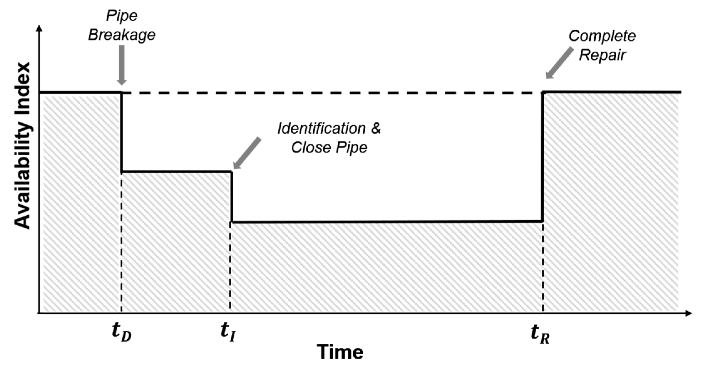
2.2. Resilience Measures

In this study, two resilience measures were used: (1) hydraulic resilience ( R H y d ) and (2) economic consequence resilience ( R E C L I P S ). Both were applied to the same failure scenario (e.g., pipe breakage), but R H y d considered hydraulic loss and R E C L I P S considered economic consequence. To make hydraulic loss and economic consequence dimensionless and on the same scale, both were normalized to be in the range of 0 and 1. The R H y d was calculated using the availability index (AI) introduced by Zhuang et al. [29], and R E C L I P S was calculated with the same AI modified with the ECLIPS factor as follows:
H A I t = i = 1 n n o d e Q i , t , d e l i = 1 n n o d e Q i , t , r e q
E A I t = i = 1 n n o d e E C L I P S i · Q i , t , d e l i = 1 n n o d e E C L I P S i · Q i , t , r e q
where, H A I t and E A I t = hydraulic and economic consequence AI, respectively; n n o d e = number of demand nodes; and Q i , t , r e q and Q i , t , d e l = required demand and delivered demand, respectively, in gpm (gallons per minute). It is important to note that the PDA model was necessary for the calculation of HAI and EAI because the unmet demand must be determined by EPANET. Both R H y d and R E C L I P S were calculated by the average of either HAI or EAI accordingly for a given simulation time as shown in Figure 1:
R H y d = t = 0 t R D H A I t   d t / t R D
R E C L I P S = t = 0 t R D E A I t   d t / t R D
where t R D = simulation time in hour, which is summation of detection time ( t I D ) and repair time ( t R I ). Expected detection time [30] was used as the detection time for pipe breakage and repair time was calculated from Walski and Pelliccia [31]:
t R I = 6.5 D 0.285
where, t R I = the repair time in hours; and D is the diameter in inches.

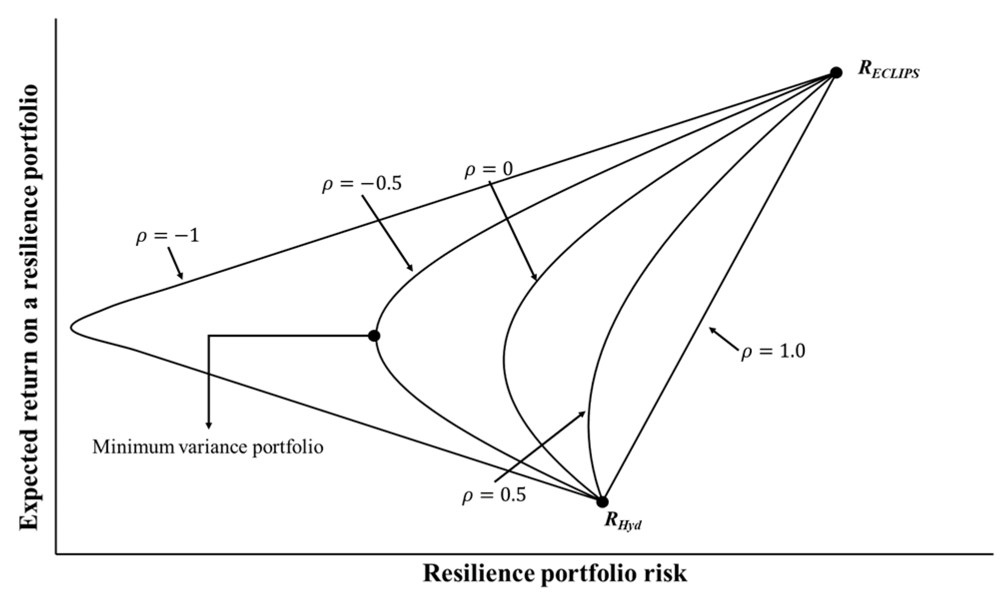
2.3. Modern Portfolio Theory

MPT originated based on the work of Harry Markowitz in the 1950s [32]. This approach has been widely used to establish the optimal investment strategies of different assets under uncertainty [33,34,35]. Portfolio theory has been applied in water resources engineering when decision-making among multiple investments is required. For example, [33] determined different flood management options using MPT, and Kidson et al. [36] and Shin and Park [34] discussed optimal allocation of diversified water resources. Climate change has been considered as an uncertain factor in determining different investment options of irrigation water demand management [35] or integrated water resources management [33]. Kang and Lansey [37] and Kang and Lansey [38] applied portfolio theory to their scenario-based multi-objective robust optimization for planning decentralized water reclamation. MPT has not been applied to guide WDS asset management using two resilience objectives.
Herein, a portfolio is defined as the set of two measures of WDS asset performance ( R H y d and R E C L I P S ), both of which can be the target for investment. MPT provides a theoretical approach to find the combination of improvement to the two resilience measures from investment in each that reduces the overall risk or increases the expected return of the portfolio [33,35].
The first step of MPT is establishing the expected return of asset performance and risks on individual assets performance. The expected return of asset performance for all m investment options can be estimated as follows:
E ( R h y d ) = k = 1 m p k · R H y d , k
E ( R E C L I P S ) = k = 1 m p k · R E C L I P S , k
where, E ( R H y d ) and E ( R E C L I P S ) = expected return of asset performance; p k = probability of a scenario k ( k = 1 , , m ); R H y d , k and R E C L I P S , k = return of asset performance of a scenario k ; and m = total number of possible scenarios. In this study, scenarios were combinations of the replacement of individual pipes and failures of individual pipes (e.g., pipe 1 replacement-pipe 1 break, pipe 1 replacement-pipe 2 break, …, pipe 2 replacement-pipe 1 break, pipe 2 replacement-pipe 2 break, so on), so m equals to the square of the number of pipes. For each scenario, return of both R H y d and R E C L I P S was calculated to get the expected return of asset performance. All scenarios had the same p k .
In MPT, a portfolio with high variance of asset performance is considered riskier mainly due to the high probability of an unexpected unfavorable return [35]. In this manner, the risk of MPT is expressed as the standard deviation:
σ H y d = S Q R T ( k = 1 m p k [ R H y d , k E ( R H y d ) ] 2 )
σ E C L I P S = S Q R T ( k = 1 m p k [ R E C L I P S , k E ( R E C L I P S ) ] 2 )
MPT investigates the expected return and risk of a portfolio along with the weight of each investment option in the portfolio. The expected return on a portfolio is a weighted average of the expected returns of each investment option as follows:
E ( R p ) = w H y d · E ( R H y d ) + w E C L I P S · E ( R E C L I P S )
where, E ( R p ) = expected return on a resilience portfolio; R p = resilience portfolio; and w H y d and w E C L I P S = weight of asset performances (the sum of the weights is one). The risk of a resilience portfolio can be evaluated as follows:
σ p = S Q R T ( w H y d 2 · σ H y d 2 + w E C L I P S 2 · σ E C L I P S 2 + w H y d · w E C L I P S · σ H y d · σ E C L I P S · ρ )
where, σ p = resilience portfolio risk; and ρ = covariance of R H y d return and R E C L I P S return but with a range from −1 to 1. In this study, covariance was measured using Pearson Correlation Coefficient (PCC).
The last step of MPT application is to determine resilience portfolios with non-inferior sets of asset performances, which produces the maximum expected return on a resilience portfolio for a given resilience portfolio risk or the minimum resilience portfolio risk for a given resilience portfolio. Figure 2 shows the example of an efficient frontier for different covariance values between R H y d return and R E C L I P S return. The point labeled “ R H y d ” is where 100% weight is assigned to R H y d , whereas “ R E C L I P S ” point is 100% weight assigned to R E C L I P S . The curves, i.e., efficient frontier consisting of non-inferior resilience portfolios, can be produced by varying weights assigned to the elements of the portfolio (keeping the sum equal to one). Generally, decision makers (investors) choose a resilience portfolio from the efficient frontier, based on their preference [39].
As shown in Figure 2, the shape of the efficient frontier is dependent on covariance. According to MPT, the risk is reduced when R H y d return and R E C L I P S return moves imperfectly about each other [32,35]. In other words, if covariance is low, such diversification can even eliminate the resilience portfolio risk [32]. The efficient frontier with the highest covariance (= 1.0) is a straight line meaning there is no diversification. On the other hand, lower covariance has a concave shaped curve indicating a more diversified resilience portfolio that reduces the resilience portfolio risk. As numerous combinations of weights exist, i.e., shares of the expected resilience portfolio and the resilience portfolio risk, the goal is to identify the share with an acceptable level of expected resilience portfolio or resilience portfolio risk. Among these options, the point at the left end (circle presented on the ρ = −0.5), where the resilience portfolio risk is minimum was identified as the minimum variance portfolio.

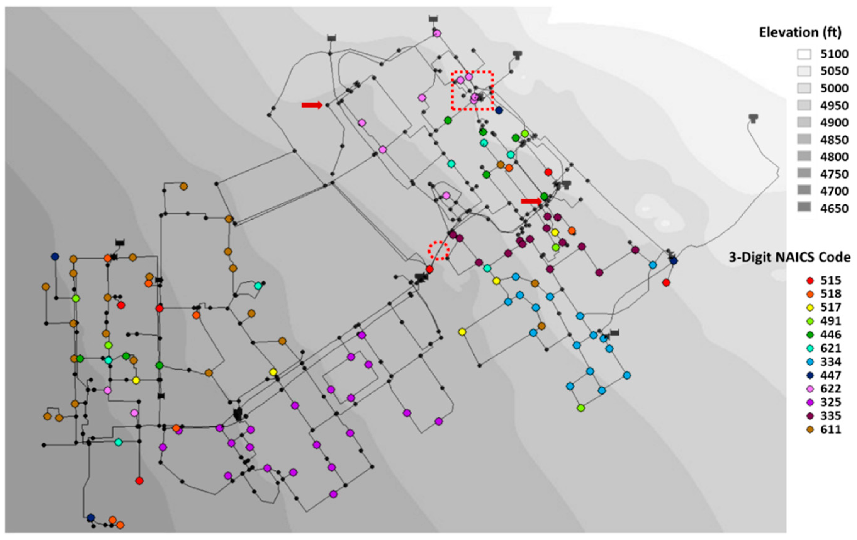
2.4. Study Network Description

The approach was tested using a WDS for a hypothetical urban area, named U-City (Figure 3). U-City represented the physical characteristics of a real network, but NAICS codes were assigned for each demand node to represent the composition of water demands in a CII portion of a city that would suffer economic consequence from reduced level of service in a WDS. The WDS had 496 pipes and 432 demand nodes. The network represented only the transmission and major distribution lines, with the majority of pipe diameters ranging from 4 inches to 16 inches. The network was supplied by five reservoirs. The network had five tanks, which can store up to 3 days of water demand for the entire system. A minimum pressure of 40 psi was a constraint at each node in the network. The system managers were concerned with aging assets, especially pipes. The average age of pipes in the system was 61 years, while the maximum age was 140 years. NAICS codes used for the network, corresponding ECLIPS, and demand for U-City WDS were adapted from Lee et al. [22] and summarized in Table 1.

2.5. Demonstrations

The case study included two demonstrations. It is worthwhile to highlight that the demonstrations were fundamental analysis of criticality for a single pipe failure and replacement scenarios designed to specifically address planning for replacement due to breakage from aging. In the first demonstration, a typical hydraulic modeling analysis was used to demonstrate the ability of R E C L I P S to provide insight complementary to R H y d . The demonstration was set for two different analyses that represent ways to plan for which pipe or pipes in a network to replace based on R H y d and R E C L I P S as the criticality measures. In the analysis, each pipe in the network was replaced with a new pipe and a steady-state simulation was executed to calculate R H y d and R E C L I P S . In a second analysis, each pipe in the network was broken (i.e., the typical N−1 contingency) and leakage modeled in a set of steady-state simulations where the reduction of R H y d and R E C L I P S were determined to represent the risk associated with each pipe, which could then be used to identify criticality.
In the pipe replacement analysis, the roughness of the replaced pipe was updated in each EPANET steady-state simulation to a value equivalent to new pipe following the relationship presented by Sharp and Walski [40]:
C = 18.0 + 37.2 l o g ( e 0 + a t D )
where, C = Hazen-Williams friction coefficient; e 0 = initial height of wall roughness at the year of installation or replacement (mm); a = growth rate of roughness height (mm/year); t = year since installation or pipe replacement; and D = pipe inner diameter (mm). To apply Equation (13) to calculate new pipe roughness, a value of t = 0 was used. Only one pipe was replaced per simulation and this was repeated until all the pipes had been replaced once. Thus, the total number of simulations was equal to the number of pipes. In the pipe breakage analysis, three time periods were modeled as shown in Figure 1. In the first time period ( t D ), an artificial node modeling a leak was created at the middle of the pipe. Then an emitter coefficient to define the magnitude of leakage rate was assigned to the new node following the approach proposed by [41]. In the next time period ( t I ), the broken pipe was isolated from the system, which was represented by closing the pipe. The expected detection time of 10.87 min was used for all simulations. Finally, in the third time period ( t R ) the failed pipe was re-opened after a specified repair time with the emitter node removed and a pipe roughness representing new pipe was assigned. These three steps were conducted for each simulation of one pipe breakage. Then the process was repeated for the next pipe and so on until pipe breakage had been simulated for all pipes. Therefore, the total number of simulations for the pipe breakage analysis was equal to the number of pipes.
The results from the pipe replacement analysis and pipe breakage analysis were expected to show differences between R H y d and R E C L I P S . These differences will demonstrate that using R E C L I P S as a criticality measure will identify different pipes than when using R H y d to prioritize for replacement, in both cases. The differences will confirm that R E C L I P S as an additional objective will help analysts include the consequences of loss of functionality in addition to the loss of functionality.
In the second demonstration, the MPT was applied to a WDS asset management analysis to find the minimum variance portfolio associated with using both R H y d and R E C L I P S . The resilience portfolio identified by the combination of the replacement of individual pipes and failures of individual pipes (i.e., N−1 contingency for each pipe replacement) provided the results to sketch the efficient frontier. Therefore, the total number of simulations for the MPT correlation analysis was equal to the square of the number of pipes. The covariance in Equation (12) was calculated using covariance of the entire set of R H y d and R E C L I P S . The relative weighting assigned to R H y d and R E C L I P S were incrementally increased or decreased by 5% while maintaining their sum at 1.0. Also, the resulting prioritization schemes for pipe replacement using R H y d only, R E C L I P S only, and the weighted combination of R H y d and R E C L I P S based on the determined minimum variance portfolio were compared using the Spearman’s rank correlation coefficient.

3. Results and Discussion
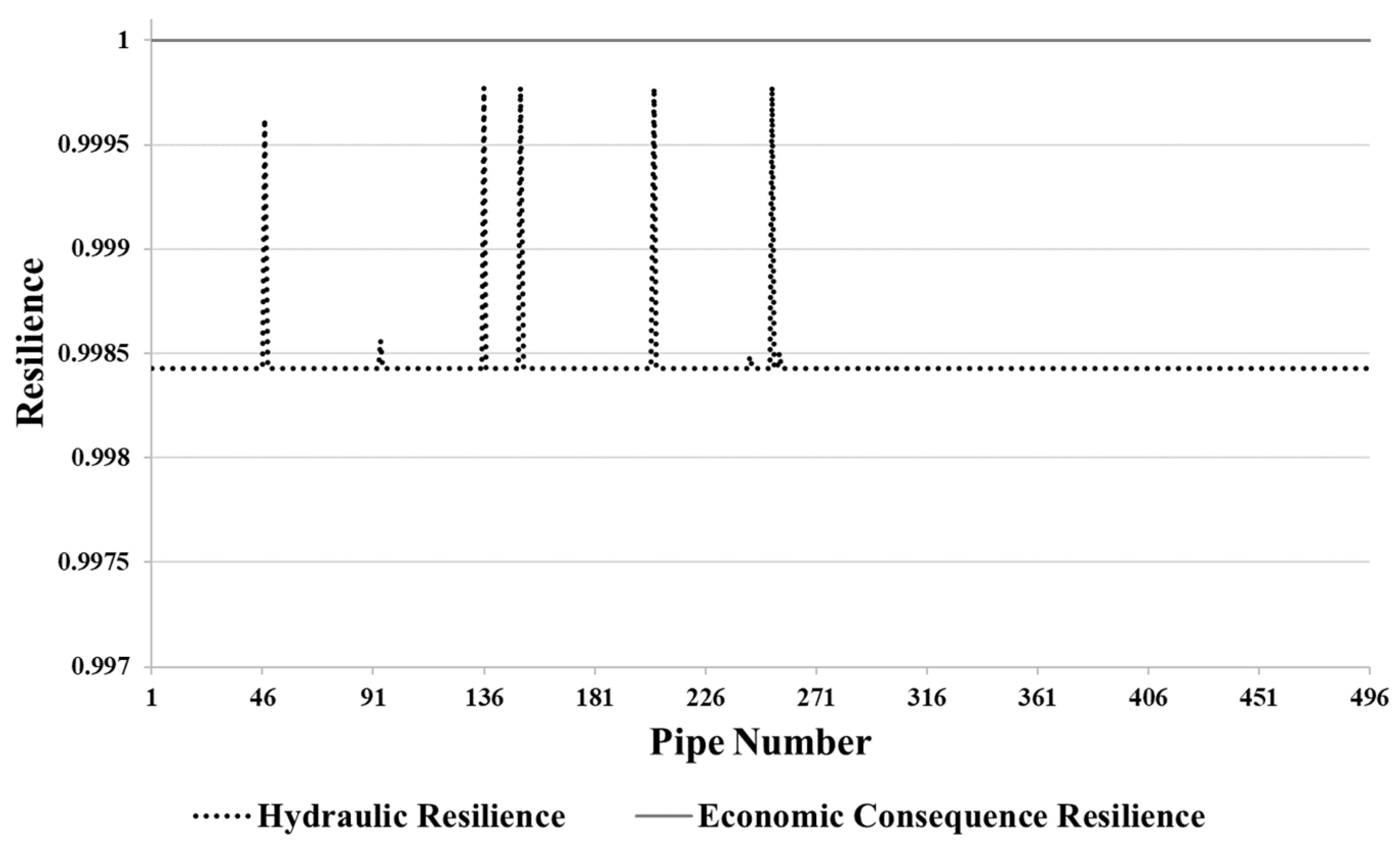
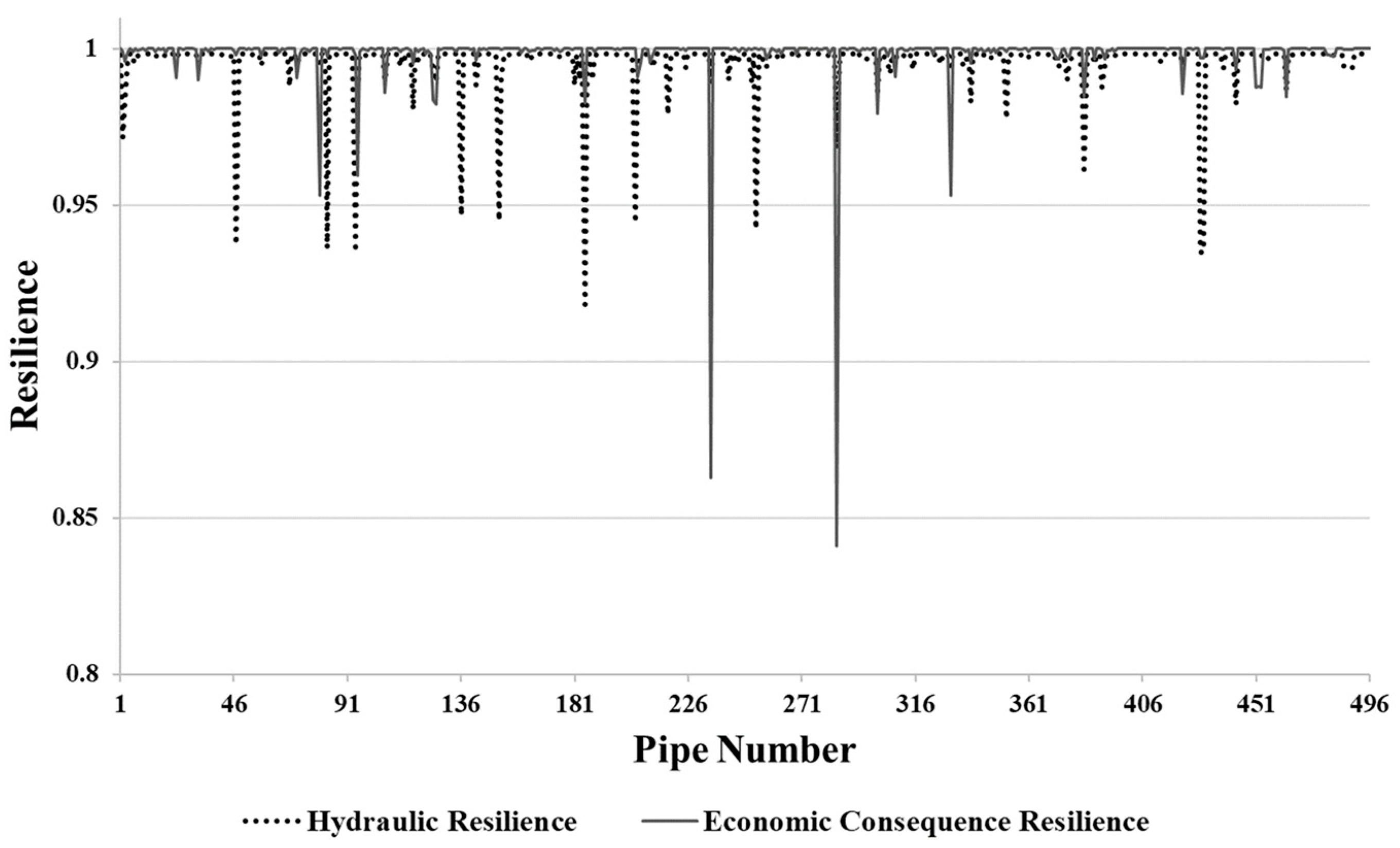
3.1. Assessment of Differences Between R E C L I P S and R H y d for Identifying Pipes Critical for Replacement

Figure 4 shows the R H y d and R E C L I P S results for the 496 pipe replacement simulations. The R H y d and R E C L I P S values (y-axis) are plotted for each pipe being replaced (x-axis). The results show that using R H y d will identify five critical pipes for replacement. Replacing these pipes would increase the resilience above the baseline of 0.998. Note that 0.0005 difference (gridline of y-axis) of R H y d will have approximately 2.55 gallons of additional water shortage in the system per minute, and $263.66 loss per minute for the same degree of R E C L I P S change for the U-City network. Using R E C L I P S proves problematic for this one case because there are no instances of insufficient pressure at a demand node supplying water for economic gain. There are two locations with insufficient pressure before replacement, and these are identified in Figure 3 with an arrow. These nodes are assigned NAICS code of 000 meaning they do not have economic value associated with the water use (i.e., that have 000 as 3-digit NAICS code, and thus, the R E C L I P S is 1 even without any replacement).
Figure 5 presents the results of resilience measures for pipe breakage (N−1 contingency) without any replacement. Based on the results, an analyst might choose the desired threshold of reduction in resilience from a pipe break to be 0.04. This would lead to identification of pipes 47, 83, 94, 136, 151 185, 205, 253, 429, and 430 when using R H y d and pipes 80, 95, 235, 285, and 330 when using R E C L I P S . There is no overlap in identified pipes from the two measures. The lowest value of R E C L I P S (the highest reduction (16%) in economic resilience) is associated with a break of Pipe 285 (dotted circle in Figure 3). This pipe delivers water to node 265, which has the highest ECLIPS (NAICS code of “515”). The R H y d value is relatively low and does not exceed the threshold because there is a relatively small demand at node 265. The largest difference between R H y d and R E C L I P S reductions from pipe breakage occurs when pipes 429 and 430 break (pipes identified by dotted rectangles in Figure 3). The hydraulic resilience decreases significantly from pipe breakage because the demand is relatively high. However, the economic consequence is relatively small because the associated NAICS code of “622” has a relatively small value. In general, the results confirm the expectation that a larger reduction in R H y d will be associated with pipes serving nodes with high demands, whereas the larger reduction in R E C L I P S will be associated with breakage to pipes serving demand nodes with a high ECLIPS. The results also show the R E C L I P S reduction is more sensitive to pipe breakage than R H y d reduction. Overall, the covariance between R H y d and R E C L I P S is found to be very low (0.2), confirming the complementary insight that may be achieved by including the economic consequence objective. Using R H y d alone to identify critical pipes for replacement may lead to increased economic consequences from pipe failure.

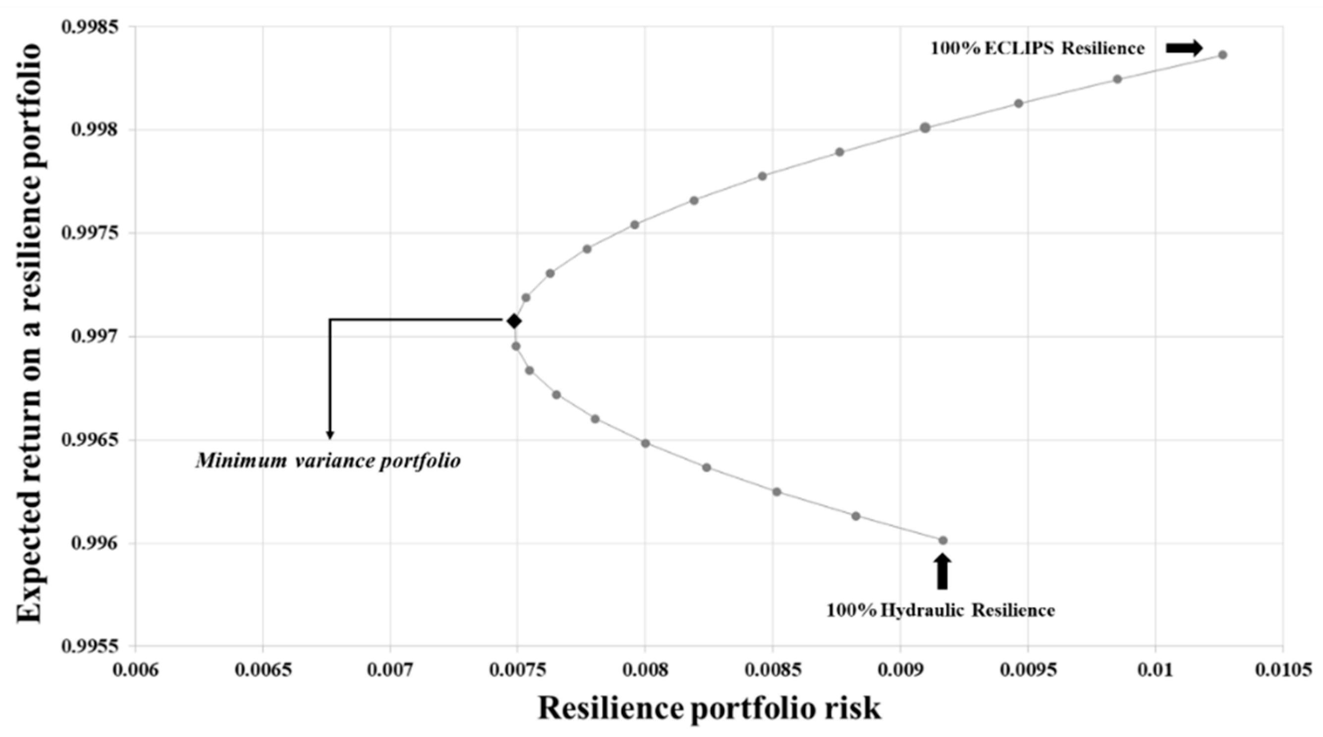
3.2. Applying Modern Portfolio Theory to Identify Minimum Combined Risk for R H y d and R E C L I P S

Figure 6 shows the efficient frontier by changing the weights assigned to R H y d and R E C L I P S . The x-axis is the resilience portfolio risk calculated using Equation (12) with covariance of 0.2 based on the MPT correlation analysis. As lower risk is preferred, the leftmost point (minimum variance portfolio) is desired. The y-axis is the expected return on a resilience portfolio, which is calculated using Equation (11). As shown in Figure 6, portfolios on the lower and upper point of the efficient frontier represents portfolios consisting of 100% of R H y d and 100% R E C L I P S , respectively. The other points represent a unique combination of weights for R H y d and R E C L I P S . For example, the point next to the R H y d of 100% has 95% weight for R H y d and 5% weight for R E C L I P S . Since WDS criticality analysis has typically used hydraulic measures, 100% weight for R H y d would be representative of ‘business as usual’.
Using the efficient frontier, a decision-maker can select the desired portfolio (i.e., weights for the two resilience measures) on the efficient frontier based on defined objectives of minimizing risk and maximizing return. The point shown as a black diamond in Figure 6 is the minimum risk (minimum variance portfolio), which has a R H y d weight of 55% and a R E C L I P S weight of 45%. The risk of this minimum variance portfolio is 0.0074, while 100% R H y d and 100% R E C L I P S have 0.0092 and 0.0103, respectively. Since the risk on the portfolio in MPT is defined as the standard deviation of the expected return on the portfolio, the larger the risk the more unlikely to achieve a target return. To help comprehend the results, it is important to note that 0.0005 difference in resilience (gridline of y axis and x axis) equates to 2.55 gallons of water loss per minute and approximately $264 loss of ECLIPS per minute. The difference of risk between 100% R H y d and the minimum variance portfolio is 10.2 gallons of water loss or $1,056 lost per minute.
Figure 7 displays a plot of how priorities of each pipe considering only R H y d or R E C L I P S relate to the priority based on the minimum variance portfolio. The spearman rank correlation coefficient between the priorities for minimum variance portfolio and R H y d or R E C L I P S is 0.91 and 0.67, respectively. As noted in the prioritized pipe analysis (Table 2), there is a strong correlation between minimum variance portfolio and R H y d , and an important yet less strong correlation with R E C L I P S . Not shown, the correlation coefficient between priorities based on R H y d or R E C L I P S is 0.53, which is relatively low.
Table 2 summarizes the top 20 pipes prioritized for replacement by the minimum variance portfolio, and shows the corresponding priority of replacement when using only the R H y d or R E C L I P S . The results show that for the most part using R H y d independently would give the same result as using the minimum variance portfolio. However, there are several important exceptions that demonstrate the benefit of including both measures. For instance, pipe 31 has a low hydraulic resilience loss, but a significant economic consequence loss. The pipe was prioritized by the minimum variance portfolio, but would have been neglected using only hydraulic resilience. Also, pipes 75, 349, 118, 32, and 309 have lower hydraulic resilience loss and would not have been ranked in the top 20 for priority, but the inclusion of the economic consequence makes them a priority for replacement.

4. Conclusions and Summary

In this study, the benefit of combining economic consequence loss with hydraulic loss using MPT to identify critical pipes for asset management was assessed. In the approach demonstrated, economic consequence loss was quantified using the ECLIPS factor based on 3-digit NAICS code categories. The case study included two demonstrations: (1) assessment of differences between R E C L I P S and R H y d for identifying pipes critical for replacement based on the correlation analysis and (2) applying MPT to identify minimum combined risk for R H y d and R E C L I P S . The demonstration used a hypothetical WDS to conduct a criticality analysis identifying pipes prioritized for replacement.
The correlation analysis confirmed that R H y d and R E C L I P S have a weak correlation (covariance of 0.2). Considering only R H y d for prioritizing pipes may lead to missing significant economic loss associated with high value users in the commercial and industrial sector. This conclusion is mainly due to a different distribution of the importance of the two resilience, demand and ECLIPS, for R H y d and R E C L I P S , respectively. Thus, an alternative approach was concluded to be needed to consider two different aspects simultaneously, which is provided by MPT in this study. The MPT demonstration results identified 55% R H y d and 45% R E C L I P S as the minimum variance portfolio. Considering 100% of R H y d as the representative of ‘business as usual’, the minimum variance portfolio would provide a benefit of saving per minute 10.2 gallons of water and $1,056 of economic productivity from use. Moreover, the minimum variance portfolio was found to prioritize pipes providing service to both high demand nodes and high economic productivity nodes, compared to using only R H y d or R E C L I P S Of the highest priority 20 pipes identified for replacement by the minimum variance portfolio, several would not have been included if only based on R H y d or R E C L I P S .
In sum, this study successfully demonstrated the approach to combine measures of economic consequence resilience with hydraulic resilience, using the MPT approach, to identify critical assets. Although the study introduces a new method to combine two resilience measures, there remain questions to address in the future. First, the probability of the scenario (pipe replacement or breakage) should be incorporated. This study assumed the probability of all scenarios to be equal. However, pipe breakage probability may differ based on material, age, length, etc. Such probability will improve the accuracy of expected return and risk for actual cases. Also, additional considerations can be studied such as multiple pipe failures and multiple pipe replacements in a group. Lastly, the method quantifying expected risk and return can be improved by considering more comprehensive coverage of the available solutions using random sampling such as Monte Carlo. As ASCE has indicated, inefficient projects may cause significant societal loses (economic consequence) compared to direct public cost (investment) [3]. This study provides a useful approach demonstrating the utility of considering economic consequence for critical asset identification.

Author Contributions

Conceptualization, S.L. and S.J.B.; Methodology, S.L. and S.S.; Validation, S.S., S.J.B., D.R.J., and T.M.; Formal analysis, S.L.; investigation, S.L. and S.S.; Resources, D.R.J., T.M.; Writing—original draft preparation, S.L. and S.J.B.; Writing—review and editing, S.L., S.J.B., and S.S.; Visualization, S.L.; Supervision, S.J.B., D.R.J. and T.M.; Project administration, D.R.J. and T.M.

Funding

This research was funded by Pacific Northwest National Laboratory (PNNL)_contract number 286187. And the APC was funded by the University of Utah.

Acknowledgments

This research was supported by the Pacific Northwest National Laboratory (PNNL). PNNL is operated for DOE by Battelle Memorial Institute under contract DE-AC05-76RL01830.

Conflicts of Interest

The authors declare no conflict of interest.

References

  1. American Water Works Association. The State of Water Loss Control in Drinking Water Utilities; White Paper; American Water Works Association: Denver, CO, USA, 2014. [Google Scholar]
  2. Solley, W.B.; Pierce, R.R.; Perlman, H.A. Estimated Use of Water in the United States in 1995; US Geological Survey: Reston, VA, USA, 1998.
  3. American Society of Civil Engineers. Failure to Act: Closing the Infrastructure Investment Gap for America’s Economic Future; American Society of Civil Engineers: Reston, VA, USA, 2016. [Google Scholar]
  4. American Society of Civil Engineers. 2017 Report Card for America’s Infrastructure; American Society of Civil Engineers: Reston, VA, USA, 2017. [Google Scholar]
  5. Little, R.G. Controlling cascading failure: Understanding the vulnerabilities of interconnected infrastructures. J. Urban Technol. 2002, 9, 109–123. [Google Scholar] [CrossRef]
  6. U.S. Environmental Protection Agency. Asset Management: A Best Practices Guide; EPA 816-F-08-014; U.S. Environmental Protection Agency: Washington, DC, USA, 2008.
  7. Boulos, P.F. Optimal Scheduling of Pipe Replacement. J. Am. Water Works Assoc. 2017, 109, 42–46. [Google Scholar] [CrossRef]
  8. Piratla, K.R.; Ariaratnam, S.T. Criticality analysis of water distribution pipelines. J. Pipeline Syst. Eng. Pract. 2011, 2, 91–101. [Google Scholar] [CrossRef]
  9. Luong, H.T.; Nagarur, N.N. Optimal maintenance policy and fund allocation in water distribution networks. J. Water Resour. Plan. Manag. 2005, 131, 299–306. [Google Scholar] [CrossRef]
  10. Alvisi, S.; Franchini, M. Near-optimal rehabilitation scheduling of water distribution systems based on a multi-objective genetic algorithm. Civ. Eng. Environ. Syst. 2006, 23, 143–160. [Google Scholar] [CrossRef]
  11. Giustolisi, O.; Berardi, L. Prioritizing pipe replacement: From multiobjective genetic algorithms to operational decision support. J. Water Resour. Plan. Manag. 2009, 135, 484–492. [Google Scholar] [CrossRef]
  12. Roshani, E.; Filion, Y. Event-based approach to optimize the timing of water main rehabilitation with asset management strategies. J. Water Resour. Plan. Manag. 2013, 140, 04014004. [Google Scholar] [CrossRef]
  13. Neelakantan, T.; Suribabu, C.; Lingireddy, S. Optimisation procedure for pipe-sizing with break-repair and replacement economics. Water SA 2008, 34, 217–224. [Google Scholar]
  14. Suribabu, C.; Neelakantan, T. Sizing of water distribution pipes based on performance measure and breakage-repair-replacement economics. ISH J. Hydraul. Eng. 2012, 18, 241–251. [Google Scholar] [CrossRef]
  15. Shamir, U.; Howard, C.D. Reliability and risk assessment for water supply systems. In Proceedings of the Computer Applications in Water Resources, Buffalo, NY, USA, 10–12 June 1985; pp. 1218–1228. [Google Scholar]
  16. Moglia, M.; Burn, S.; Meddings, S. Decision support system for water pipeline renewal prioritisation. J. Inf. Technol. 2006, 11, 237–256. [Google Scholar]
  17. Shin, S.; Lee, S.; Judi, D.R.; Parvania, M.; Goharian, E.; McPherson, T.; Burian, S.J. A Systematic Review of Quantitative Resilience Measures for Water Infrastructure Systems. Water 2018, 10, 164. [Google Scholar] [CrossRef]
  18. Hosseini, S.; Barker, K.; Ramirez-Marquez, J.E. A review of definitions and measures of system resilience. Reliab. Eng. Syst. Saf. 2016, 145, 47–61. [Google Scholar] [CrossRef]
  19. Jayaram, N.; Srinivasan, K. Performance-based optimal design and rehabilitation of water distribution networks using life cycle costing. Water Resour. Res. 2008, 44. [Google Scholar] [CrossRef]
  20. Jin, H.; Piratla, K.R. A resilience-based prioritization scheme for water main rehabilitation. J. Water Supply Res. Technol. 2016, 65, 307–321. [Google Scholar] [CrossRef]
  21. Chang, S.E.; Svekla, W.D.; Shinozuka, M. Linking infrastructure and urban economy: Simulation of water-disruption impacts in earthquakes. Environ. Plan. B Plan. Des. 2002, 29, 281–301. [Google Scholar] [CrossRef]
  22. Lee, S.; Shin, S.; Judi, D.; McPherson, T.; Burian, S. Water Distribution System Recovery Strategies Considering Economic Consequences from Business Loss. In Proceedings of the CCWI2017, Sheffield, UK, 5–7 September 2017. [Google Scholar]
  23. Rossman, L.A. EPANET 2: Users Manual; U.S. Environmental Protection Agency: Washington, DC, USA, 2000.
  24. Judi, D.R.; McPherson, T.N. Development of Extended Period Pressure-Dependent Demand Water Distribution Models; Los Alamos National Lab.(LANL): Los Alamos, NM, USA, 2015.
  25. Heflin, C.; Jensen, J.; Miller, K. Understanding the economic impacts of disruptions in water service. Eval. Program Plan. 2014, 46, 80–86. [Google Scholar] [CrossRef]
  26. Pagsuyoin, S.A.; Santos, J.R.; Chua, L.; Irvine, K. Modeling the effects of drought in urban economies using regional input-output analysis. Int. J. Environ. Clim. Chang. 2015, 5, 134–146. [Google Scholar] [CrossRef]
  27. Federal Emergency Management Agency. Hazard Mitigation Assistance Unified Guidance; Federal Emergency Management Agency: Washington, DC, USA, 2010.
  28. U.S. Department of the Interior Bureau of Reclamation. Cataloguing Commercial, Industrial, and Institutional Customer Classes. 2009; Volume 2 of 5. Available online: https://www.usbr.gov/lc/socal/reports/weep/Vol2CIIcustomers.pdf (accessed on 08 October 2018).
  29. Zhuang, B.; Lansey, K.; Kang, D. Resilience/availability analysis of municipal water distribution system incorporating adaptive pump operation. J. Hydraul. Eng. 2012, 139, 527–537. [Google Scholar] [CrossRef]
  30. Lee, S.; Shin, S.; Judi, D.; McPherson, T.; Burian, S. Detectability-Based Resilience of Water Distribution System Using Failure Finger Print. In Proceedings of the WDSA/CCWI Joint Conference 2018, Kingston, ON, Canada, 23–25 July 2018. [Google Scholar]
  31. Walski, T.M.; Pelliccia, A. Economic analysis of water main breaks. J. Am. Water Works Assoc. 1982, 74, 140–147. [Google Scholar] [CrossRef]
  32. Markowitz, H. Portfolio selection. J. Financ. 1952, 7, 77–91. [Google Scholar]
  33. Aerts, J.C.; Botzen, W.W.; Werners, S.E. Portfolios of adaptation investments in water management. Mitig. Adapt. Strateg. Glob. Chang. 2015, 20, 1247–1265. [Google Scholar] [CrossRef]
  34. Shin, S.; Park, H. Achieving cost-efficient diversification of water infrastructure system against uncertainty using modern portfolio theory. J. Hydroinform. 2018, 20, 739–750. [Google Scholar] [CrossRef]
  35. Paydar, Z.; Qureshi, M. Irrigation water management in uncertain conditions—Application of Modern Portfolio Theory. Agric. Water Manag. 2012, 115, 47–54. [Google Scholar] [CrossRef]
  36. Kidson, R.; Haddad, B.; Zheng, H. Improving water supply reliability through portfolio management: Case study from Southern California. In Proceedings of the 4th WEAS International Conference in Water Resources, Hydrology and Hydraulics, Cambridge, UK, 24–26 February 2009; pp. 24–26. [Google Scholar]
  37. Kang, D.; Lansey, K. Multiperiod planning of water supply infrastructure based on scenario analysis. J. Water Resour. Plan. Manag. 2012, 140, 40–54. [Google Scholar] [CrossRef]
  38. Kang, D.; Lansey, K. Scenario-based robust optimization of regional water and wastewater infrastructure. J. Water Resour. Plan. Manag. 2012, 139, 325–338. [Google Scholar] [CrossRef]
  39. Elton, E.J.; Gruber, M.J.; Brown, S.J.; Goetzmann, W.N. Modern Portfolio Theory and Investment Analysis; John Wiley & Sons: Hoboken, NJ, USA, 2009. [Google Scholar]
  40. Sharp, W.W.; Walski, T.M. Predicting internal roughness in water mains. J. Am. Water Works Assoc. 1988, 80, 34–40. [Google Scholar] [CrossRef]
  41. Yoo, D.G.; Jung, D.; Kang, D.; Kim, J.H.; Lansey, K. Seismic hazard assessment model for urban water supply networks. J. Water Resour. Plan. Manag. 2015, 142, 04015055. [Google Scholar] [CrossRef]
Figure 1. Availability index variation to simulation time and condition.
Water 11 01222 g001
Figure 2. Efficient frontier example with different covariance.
Water 11 01222 g002
Figure 3. The layout of the U-City water distribution system (WDS). Dotted rectangle and circle highlight important locations of pipes noted later in the results that have significant loss of hydraulic resilience and economic consequence resilience. The node pointed to by the arrow is where minimum pressure is violated without any pipe replacement.
Water 11 01222 g003
Figure 4. R H y d and R E C L I P S values for all iterations of the pipe replacement analysis.
Water 11 01222 g004
Figure 5. Hydraulic and ECLIPS resilience variation under pipe breakage simulation without pipe replacement.
Water 11 01222 g005
Figure 6. Efficient frontier between hydraulic resilience and ECLIPS resilience.
Water 11 01222 g006
Figure 7. Pipe replacement priority difference to the pipe replacement priority based on the system resilience.
Water 11 01222 g007
Table 1. Candidate NAICS code for U-City and water cost information, number of the EPANET model nodes serving the NAICS code, and total demand for the nodes serving the NAICS code following Lee et al. [22].
3-Digit NAICSDescriptionECLIPS (M$/Gal)Number of NodesDemand (GPM)
515Broadcasting (except Internet)0.0282576179.71
518Internet Service Providers, Web Search Portals, and Data Processing Services0.0067808313.08
517Telecommunications0.005268541.04
491Postal Service0.002229569.33
446Health and Personal Care Stores0.0019258354.23
621Ambulatory Health Care Services0.0012547134.96
334Computer and Electronic Product Manufacturing0.00095616303.98
447Gasoline Stations0.000922418.44
622Hospitals0.00081911762.87
325Chemical Manufacturing0.00066321428.10
335Electrical Equipment, Appliance, and Component Manufacturing0.00052115317.18
611Educational Services0.00008023649.27
000Landscape Irrigation or Other Non-Revenue Generating Use0.0000003031524.00
Table 2. Comparison of priorities of the 20 pipes identified as the highest priority for replacement based on the minimum variance portfolio (i.e., weighted combination of R H y d and R E C L I P S ). Shown for comparison are the replacement priorities of the pipe based on R H y d or R E C L I P S .
PipeMVP * R H y d R E C L I P S PipeMVP * R H y d R E C L I P S
13611343347119473
20522459185121812
151334487513213
253444872561411484
47557534915277
316471111816434
24776172441712481
26088243218586
2009102330919319
9410784285204275
* MVP: Minimum variance portfolio.

