Research on Unsteady Hydraulic Features of a Francis Turbine and a Novel Method for Identifying Pressure Pulsation Transmission Path


1
College of Water Conservancy and Hydropower Engineering, Hohai University, Nanjing 210098, China
2
Powerchina Changsha Engineering Corporation Limited, Changsha 410014, China
*
Authors to whom correspondence should be addressed.
Water 2019, 11(6), 1216; https://doi.org/10.3390/w11061216
Submission received: 30 May 2019
/
Revised: 6 June 2019
/
Accepted: 10 June 2019
/
Published: 11 June 2019
(This article belongs to the Section Hydraulics and Hydrodynamics)
Abstract
:It is of significant value to understand the unsteady hydraulic features and pressure pulsation transmission path in the flow channel through a turbine for providing technical support for turbine design and optimization, as well as laying a foundation for analysis of the stability and the coupled vibration of the hydropower house. In this paper, a three-dimensional mechanics–hydraulics–concrete structure coupled numerical model was established to accurately simulate Francis hydraulic machinery, including the high-rotating turbine runner and fixed guide vane, the unsteady flowing water, the structure of the entire flow channel, as well as the dynamic interaction between them. Turbulent hydraulic features of flow condition and pressure pulsation in design operation were explored using the detached eddy simulation (DES) turbulence model. Then, a novel method was proposed to identify the fluid pressure pulsation transmission path based on the time-delayed transfer entropy method and wavelet theory. On basis of time and frequency analysis of pressure calculation results, investigation into identification of pressure pulsation transmission path was performed using the method of traditional transfer entropy and the method adopted in this paper. The pressure pulsation transmission features in the entire flow channel were revealed during operation of the large-scale Francis turbine. The research method and results could not only lay a basis for exploring the structural vibration regularity of the hydropower house but also provide a scientific reference for vibration reduction design of the hydropower house.
1. Introduction
Hydropower, one of the renewable and alternative energy sources for electricity generation, is becoming increasingly favorable with the installed unit capacity steadily increasing. The complex and changeable flow condition in hydraulic turbine, the core component in hydropower generation, including Karman vortices formed around the stay vanes, guide vanes or runner blades, and procession of vortex core in the draft tube, is responsible for hydraulic vibration in the hydropower station. Accurate and detailed description of internal flow condition and vibration features of structural components using computational fluid dynamics (CFD), computational structure dynamics (CSD), and fluid–structure interaction (FSI) guarantees successful design of high-performance hydraulic turbines. Therefore, it is of great significance to fully understand the flow characteristics in the flow channel through turbine and the dynamic interaction between the turbulence flow and the flow passing components for performance prediction and design optimization of hydraulic turbines.
CFD and CSD are considered as reliable and economic tools to analyze the performance of the turbines. Investigations have been performed for analysis of flow features in hydraulic machinery for a long time [1]. Arispe et al. [2] carried out CFD analysis of turbine performance with different draft tube geometries at the best efficiency point (BEP). The numerical results were compared with the experimental results of the reduced model corresponding to the GAMM (Gesellschaft für Angewandte Mathematik und Mechanik/Society of Applied Mathematics and Mechanics) Francis turbine. Trivedi et al. [3] investigated pressure pulsations on two prototype Francis turbines at five operating points based on statistical analysis, spectral analysis, coherence, and cross-correlation between the signals. Li et al. [4] conducted CFD analysis of the pressure pulsations in a prototype pump–turbine in turbine mode with different blade numbers. Mössinger et al. [5] investigated axial velocity distribution and pressure pulsations in the turbine during two load changes and turbine shutdown processes. Chalghoum et al. [6] analyzed the effect of the impeller diameter and number of blades on the pressure evolution in a centrifugal pump during startup process. Goyal et al. [7] discussed the flow features in a high head model Francis turbine at part load operation and found the rotating vortex rope in the draft tube caused severe fluctuations and vibrations of the draft tube.
FSI is the present-day state-of-art technique, which has increased applications in complicated hydraulic mechanical engineering. Xiao et al. [8] conducted one-way FSI analysis of flow field and static and dynamic stress in the runner of a Francis turbine and concluded that dynamic stress was a main contributor to fatigue and cracks of the blade during off-design operation. Two-way coupled FSI could consider the feedback of the blade deflection on the flow by conducting iterations between fluid and solid system. Frederick et al. [9] calculated the dynamic behavior of a Francis turbine runner under operating condition based on the two-way FSI method introduced by ANSYS (Analysis Systems) software.
Current studies of the Francis turbine mainly focus on the internal flow features, attaching little attention to the transmission path of the fluid pressure pulsation. Hydraulic vibration, as one of the most important vibration sources, plays a vital role in analysis of the coupled vibration of the hydropower house, with the potential of generating significant pulsations to threaten the safety of the powerhouse. It is of great significance to understand the regularity and transmission path of fluid pressure pulsation for guidance of safety, stability, and vibration attenuation during the unit operation.
Time-delayed transfer entropy emerged from information entropy, which was proposed by Shannon and introduced into information theory to measure information uncertainty. As an asymmetric measurement defined by Schreiber in 2000, transfer entropy contains directional and dynamic information based on definition of transition probabilities and has been well applied in the energy transfer between different information flows [10,11]. Without assuming any model in advance, transfer entropy is sensitive to the relationship of any order between systems [10], which is important to exploring the unknown nonlinear correlation. Therefore, in this paper, the time-delayed transfer entropy is introduced into the analysis of the pressure pulsation transmission path in a hydropower house.
Known as a mathematical microscope, wavelet transform is a window-adaptive time–frequency analysis method, with an automatically narrow time window at high frequency information and wide time window at low frequency information, which makes wavelet transform render higher time resolution and lower frequency resolution at high frequency information and higher frequency resolution and lower time resolution at low frequency information. Wavelet transform helps to identify the information transmission direction by extracting a single frequency component from the complex pulsation frequency components of hydraulic vibration sources.
In this paper, with currently the largest unit capacity of 800 MW in China, a three-dimensional hydraulic machinery–fluid flow–concrete structure coupled model of the Xiangjiaba hydropower house was established to perform a realistic dynamic interaction between the high-speed rotating turbine runner and the unsteady turbulent flow. Hydraulic features were accurately analyzed based on the SA-DES (Spalart-Allmaras detached eddy simulation) method and two-way iterative FSI solver as in-house codes in ADINA (Automatic Dynamic Incremental Nonlinear Analysis) software, including flow condition and pressure pulsation in the entire flow channel through a Francis turbine during design operation, which lays a firm foundation for correct identification of the pressure pulsation transmission path. Based on the self-programming code in MATLAB software, the traditional transfer entropy method and the combined transfer entropy–wavelet method adopted in this paper were compared for identifying pressure pulsation transmission direction, and the rationality and effectiveness of the proposed method were confirmed. The research results not only reveal the transmission path of pressure pulsation in the entire flow channel of the hydropower house but also render important guidance and engineering application prospects for design optimization and hydraulic performance evaluation of the Francis turbine, as well as laying a firm basis for studying the structural vibration regularity of the hydropower house.
2. Basic Theory and Numerical Model
2.1. Basic Equations
The SA–DES turbulence model was applied into unsteady turbulence treatment and better prediction of the pressure pulsation using ADINA software. Derived from the SA one-equation eddy–viscosity RANS (Reynolds-averaged Navier-Stokes) model, SA–DES combines the advantages of large eddy simulation (LES) and the RANS method and could simulate the large-scale turbulent pulsations accompanied by the precession of vortex in hydraulic machinery economically and reliably [12,13]. The one-equation DES turbulence model is expressed below [14,15,16]:
where is the working variable in the order of the molecular viscosity. The model coefficients are given by: cb1 = 0.1335, cb2 = 0.622, σ = 2/3, cω1 = cb1/k2 + (1 + cb2)/σ, , cω3 = 2, g = r + cω2(r6 − r), , cω2 = 0.3, , , , , , cν1 = 7.1.
As the switch function of the LES–SGS (large eddy simulation - sub-grid scale) and RANS turbulence model, dDES is described in the form of Equation (2):
where d is the nearest distance to the wall and Δmax is the maximum local grid size, CDES = 0.65.
On the basis of built-in features in ADINA software, both the kinematic and the dynamic condition are applied to the fluid–solid coupling interface to obtain compatible traction and displacement [17]. Corresponding equations are expressed as follows:
where and are, respectively, the fluid and solid displacements. and are the fluid and solid stresses, respectively. The underlining denotes that the values are defined only on the fluid–structure interfaces.
Transfer entropy was employed for identification of pressure pulsation path using MATLAB software. It focuses on quantification of the additional information from one state variable to the other’s transition probabilities. If the dynamic probabilities of a process x at time of n + 1 is conditional only on previous k values, the process is called a kth-order Markov process [18,19]. The mathematic description of this transition probability is p(x(n + 1)|x(n), x(n − 1), …, x(n − k + 1)) = p(x(n + 1)|x(n)(k)) = p(x(1)|x(k)). Note the n is omitted for convenience. Considering the influence of another process y(m)(l) on these transition probabilities, the expression of coupling influence of both x(n)(k) and y(n)(l) on x(n + 1) is p(x(1)|x(k), y(l)). The transfer entropy can be formulated as below [20]:
According to this equation, very high-dimensional probability densities must be solved before obtaining the transfer entropy, resulting in plenty of calculation cost. One-order of the processes (k = l = 1) has been adopted in previous studies to solve the transfer entropy for simplicity [21,22]. Together with a time delay τ added to y(n), Equation (5) can be rewritten as Equation (6), and the result can be referred to as the time-delayed transfer entropy:
where y(τ) ≡ y(n + τ). The assumption of order k = l = 1 quantifies the information gain from y(τ) only. Nevertheless, the resulting transfer entropy will not be zero if the information of process x presents within its own past history, like y = x.
In practice, due to the complicated vibration frequency components in original signals, the calculated curves of the time-delayed transfer entropy between two adjacent measuring points might be overlapped, which makes it hard to identify the vibration transmission direction. Wavelet transform could tackle this problem by extracting the time series with the specific frequency component from the original data. The combined wavelet and time-delayed transfer entropy for two stable Markov processes x and y with the scale factor a and the time delay τ is written in Equation (7):
where wx(a) is the wavelet transform of x at scale factor a. Using wavelet transform, the characteristic frequencies can be extracted from the original vibration signal. Hence, the direction of information transmission can be effectively identified on the basis of calculating the time-delayed transfer entropy of the newly obtained signal.
2.2. Numerical Simulation Model
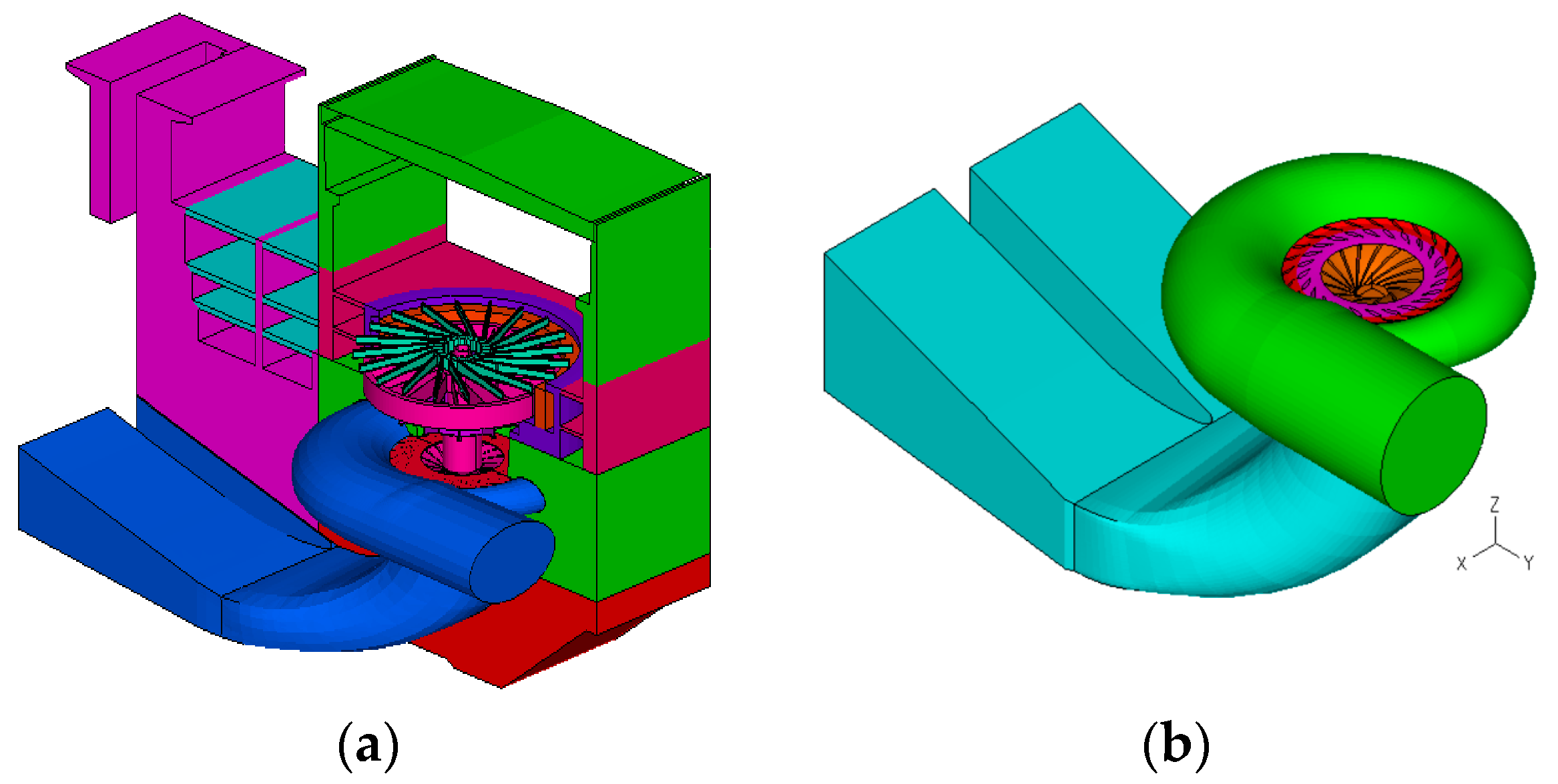
A large-scale 3D fluid–concrete structure–hydraulic machinery coupled geometric model was established based on the Xiangjiaba hydropower house owning the currently largest installed capacity of 800 MW in China, including simulations of the concrete structure of the hydropower house, mechanical structure of the hydraulic turbine, generator, upper and lower bracket, and the entire water flow inside the flow channel, as shown in Figure 1a. Simulation of the vibration energy transmission path allowed fluid pressure pulsation to transmit from the rotating runner blades to downstream and upstream components and also represented the dynamic mutual impact of transient pressure pulsation propagating among these sections. Figure 1b displays the computational model of the entire fluid domain through the turbine. The number of runner blades was 15, and the number of guide vanes was 24. The rated rotational speed of the hydraulic turbine was 75 rpm, and the specific speed was 213.7. This turbine was a medium-head turbine with a rated head H of 100 m. A uniform velocity was applied to the inlet in terms of the flow rate, and outflow was set as the outlet boundary condition.
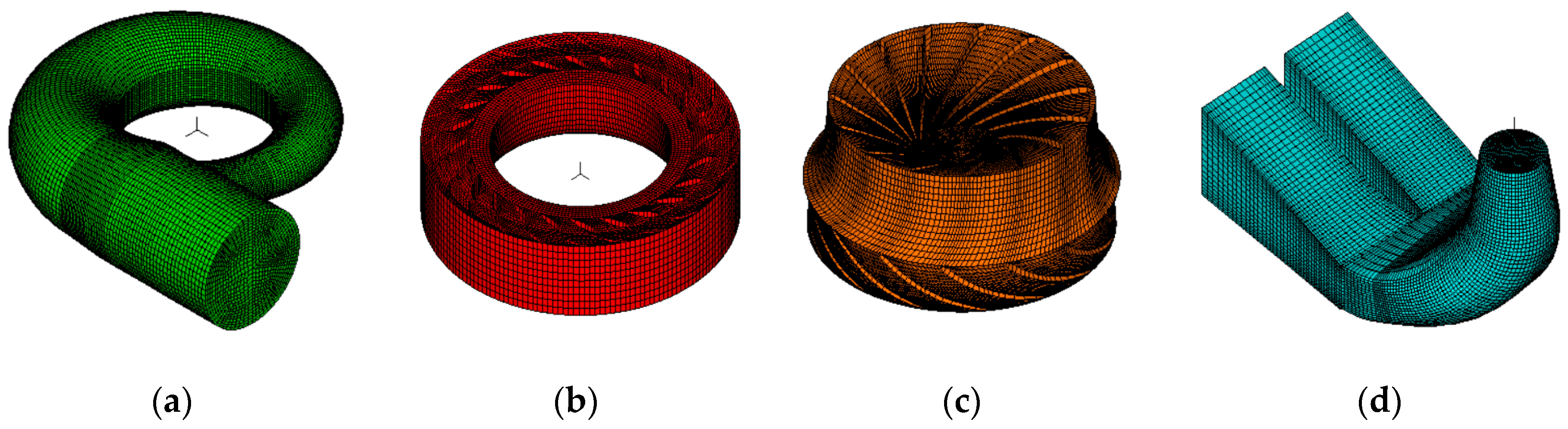
Figure 2 illustrates the structured grids for four subregions in fluid domain, involving fluid in a spiral casing, fluid around the stay vane, guide vane, and runner, and fluid in a draft tube. Finer grids were applied to the rotational zone and field near the wall in fluid domain to ensure high-accuracy results. A mesh independence test was conducted to obtain a reasonable number of computational grids, in which the head values in different grid sizes were evaluated under steady state by imposing velocity at the inlet and outflow at the outlet. The fluid domain comprises 442,704 3D-fluid elements and 481,906 grid nodes.
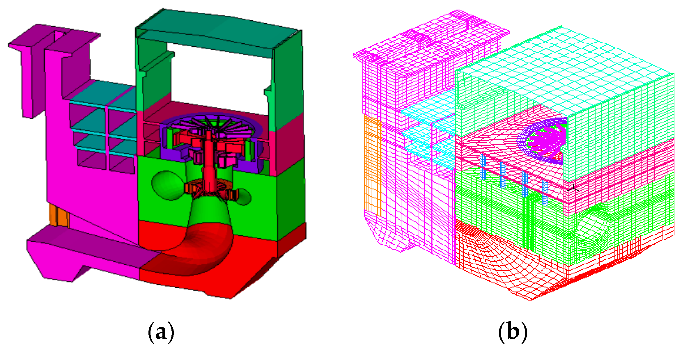
The solid geometric model and 3D structural grids are shown in Figure 3. Both the concrete structure, including the turbine floor, dynamo floor, draft tube block structure, sidewall, and roof, and the mechanical structure, including the runner, axis and rotor, upper and lower bracket, and stay and guide vane, are simulated in this research. The solid domain is composed of 187,636 elements and 136,752 grid nodes.
A simultaneous calculation was performed using the two-way iterative FSI method with the CFD solver based on the finite volume method (FVM) in fluid domain and CSD solver based on the finite element method (FEM) in solid domain. In the fluid domain model, sliding mesh boundary conditions were adopted to connect rotating domains to ensure the compatibility and continuity along the nonconforming interfaces. The FSI boundary condition was imposed on the entire interfaces between the fluid and solid model, including the interfaces between the entire water flow and the surrounding concrete, water and the rotating blades, water and the stay vanes, and water and the guide vanes. The second-order upwind scheme was applied to the governing equations of the fluid part to ensure the stability of the calculation process. In equation residual, mass convergence criteria were adopted with a tolerance of 0.0001, while in variable residual, both velocity and pressure convergence criteria were adopted, and the tolerance was 0.001. The equations were required to be converged at every time step after iteration. The total calculation time was set as 8 s, with a time step of 0.002222 s, corresponding to 1° of the runner rotation.
3. Transient Hydraulic Features in Fluid Domain
Since pressure pulsation is an external manifestation of hydraulic stability, it is of guiding significance to study pressure pulsation in the flow field of hydraulic turbines and capture its time–frequency characteristics in order to understand the evolution law of the flow field and the hydraulic stability.
In this section, since the pressure pulsation amplitude was much smaller than the static pressure value, the static pressure was eliminated from the original nodal pressure by employing pressure pulsation coefficient Cp. The equation of Cp is as follows:
where p is the static pressure; is the average static pressure of one rotational cycle of blades; ρ is the water density; and u is the peripheral velocity of blade tip.
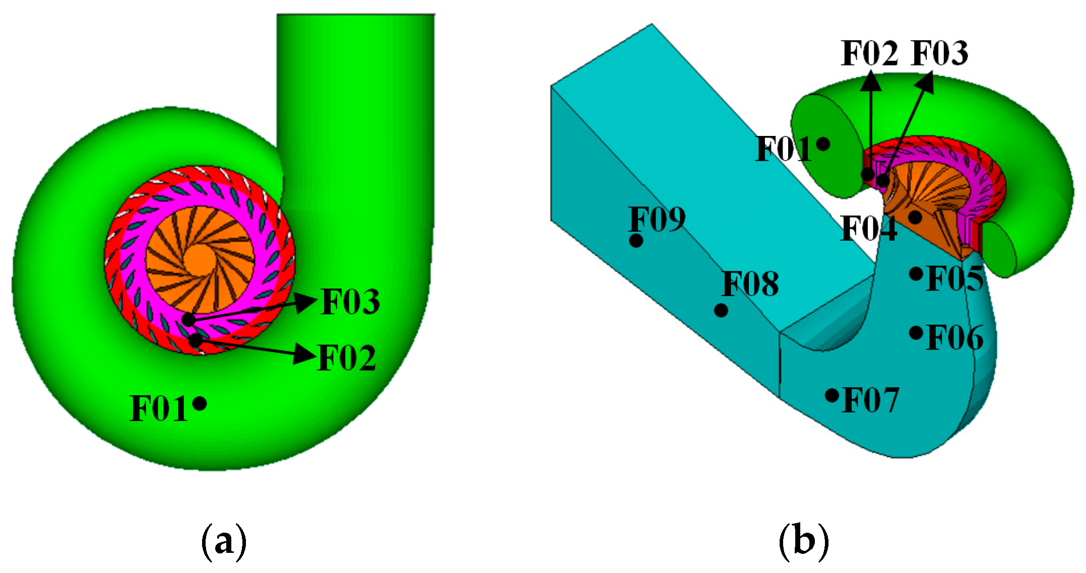
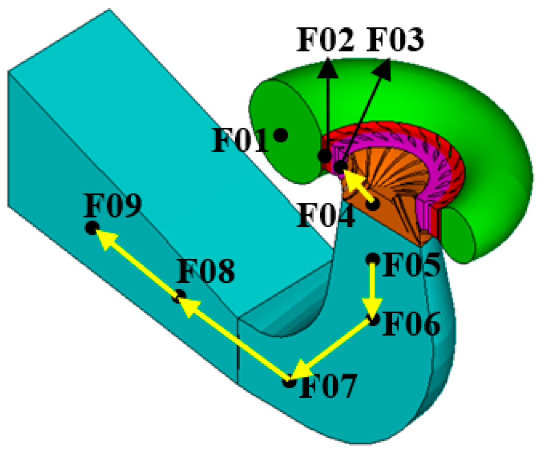
In order to analyze the time and frequency features of the pressure fluctuation, as well as its transmission law in the flow field, measuring points F01–F09 were placed at positions of spiral casing, between the stay ring and guide vane, vaneless region, 0.3 D straight cone section of draft tube, elbow section of draft tube, and diffusion section of draft tube, respectively, and the distribution of the nine measuring points is shown in Figure 4. These measuring points were placed only in the fluid region during the numerical process rather than physical measurements. Note the methodology of both transfer entropy and wavelet theory has no direct correlation with the positions of selected points, since one of the advantages of the proposed methodology is flexibility and can be applied to the points of any position.
3.1. Hydraulic Features of the Flow Field in the Spiral Casing and Vaneless Region
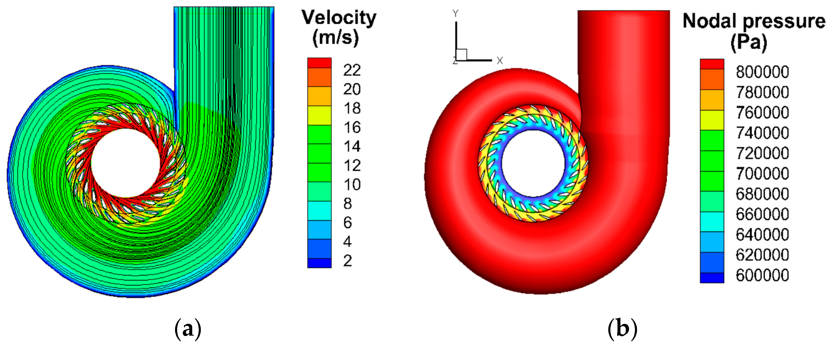
Spiral casing serving as an important diversion component of the Francis turbine is responsible for guiding the water to generate circular motion and uniform and axial symmetrical flow condition before flowing into the overflow components. Since the water flows into the high-speed rotating runner directly after flowing through the stay and guide vanes, the guide vane is the key to guiding water to form a certain velocity moment and enter the runner in a proper direction.
Figure 5 shows the velocity and pressure contour with streamline distribution in the spiral casing and vaneless region during design operation. The streamlines were continuous and smooth in the channel, and the distribution of velocity and pressure was symmetrically circumferential. The velocity increased gradually with the decrease of the radial flow section. The pressure decreased along the radial direction, with a value of about 1.0 MPa in the spiral casing. The pressure transition was smooth without obvious sudden changes. Calculation results indicated that the inflow in the circumferential direction was symmetrical enough to retain a uniform flow, and the design of the spiral casing was reasonable. The direction of the nodal pressure damping was from spiral casing to the guide vane and would be compared with the identified pulsation transmission direction in the next section.
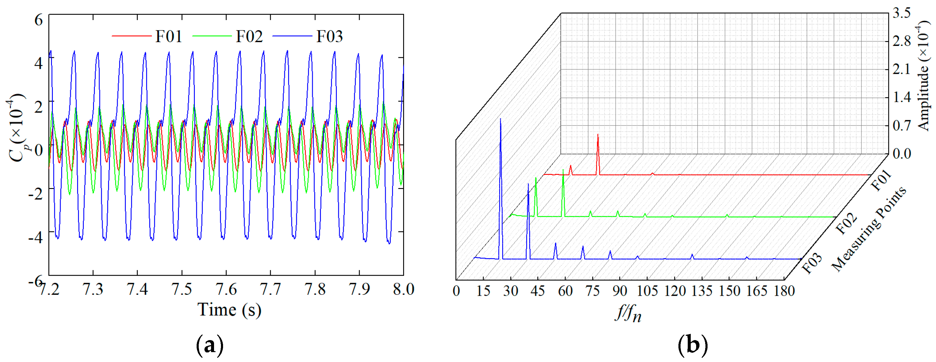
Figure 6 displays the time varying and frequency spectrum of the Cp of measuring points F01 at the spiral casing, F02 between the stay and guide vane, and F03 at the runner inlet. The pressure pulsation of the three measuring points fluctuated regularly from 7.2 to 8.0 s. The closer the position of the measuring point to the runner was, the greater the pressure fluctuation amplitude. Here, we define fn as the blade rotation frequency 1.25 Hz and 15fn as the blades passing frequency 18.75 Hz. The frequency domain diagram shows that the main frequency components of pressure pulsation were: 15fn, 30fn, and 45fn, which indicated that pressure fluctuation in spiral casing and vaneless region was mainly affected by the blades’ rotation.
3.2. Hydraulic Features of the Flow FIeld in the Runner
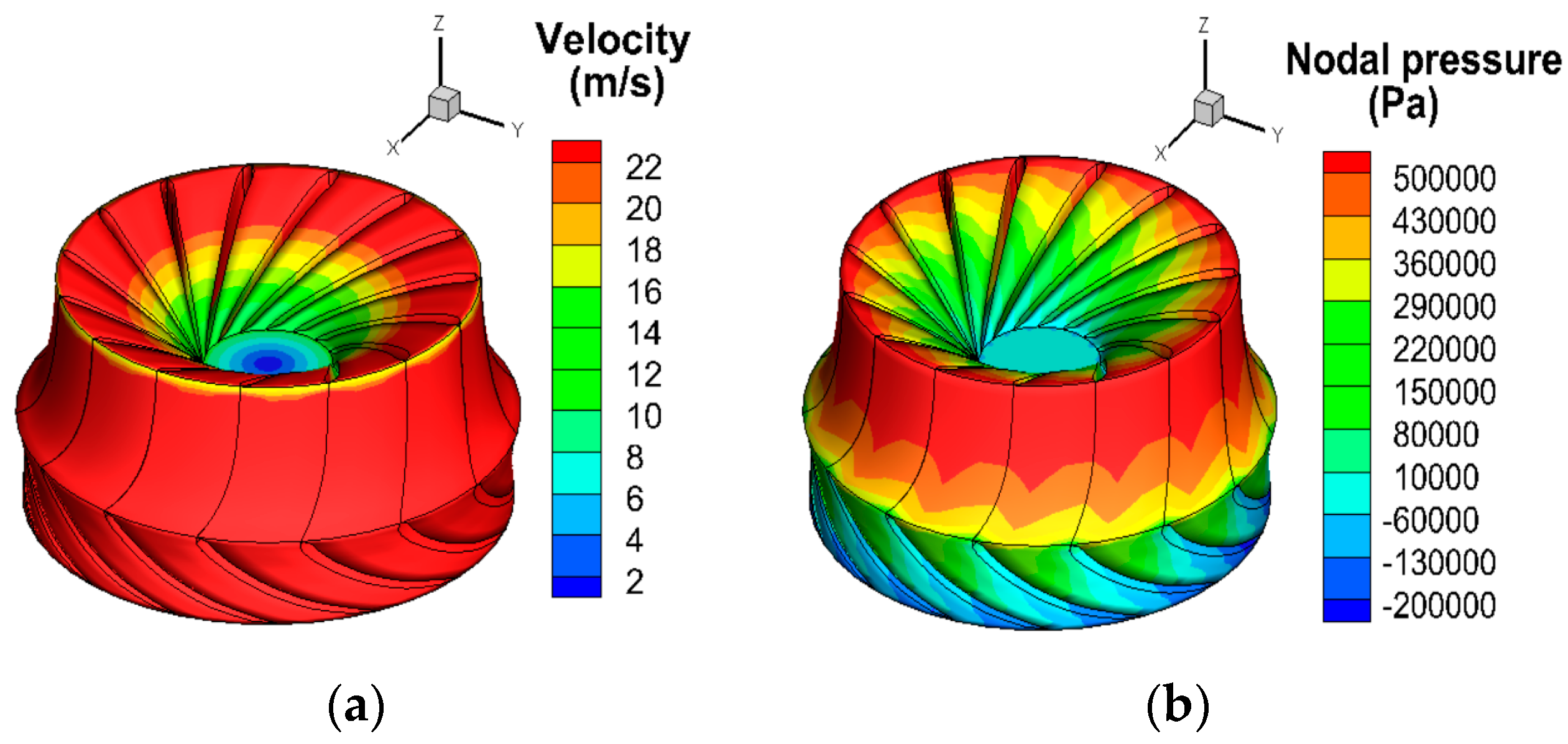
Analysis of the flow pattern in the runner plays a decisive role because the runner is the core overflow component for energy conversion. Figure 7 gives the contour of velocity and pressure in the flow field of the runner. The velocity and pressure distribution in the flow-driven rotating runner was periodically symmetric, with relatively ideal distribution of the pressure at the runner inlet. The pressure on the pressure side of the blade was higher, but on the suction side, larger negative pressure occurred, reaching about −0.2 MPa, which could easily cause blade cavitation. The relative flow direction of the water changed under the restriction of the blades when the water entered into the runner chamber. At the same time, the water tried to keep the original flow direction and resisted the restriction of blades due to the motion inertia. Under these two conditions, the mechanical energy of the flowing water can be transformed into that of the rotating runner.
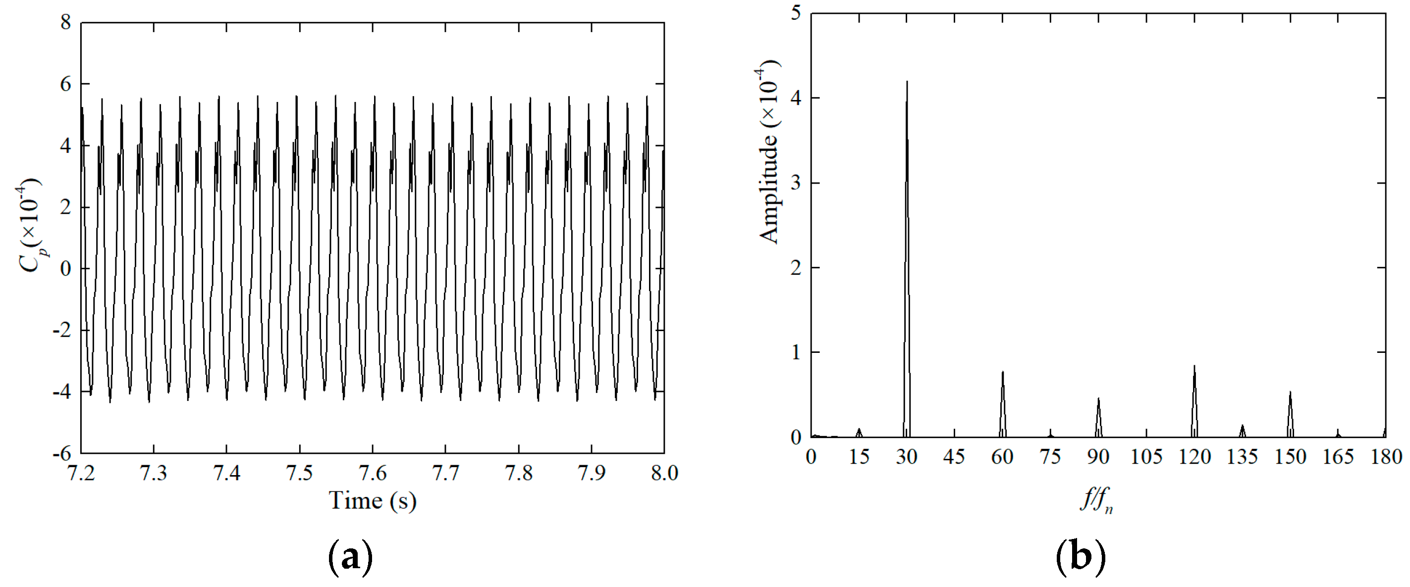
The time and frequency domain diagram of Cp at the measuring point F04 is illustrated in Figure 8. It is clearly seen that the pressure in the runner chamber fluctuated regularly with the higher pulsation amplitude. Frequency domain analysis in Figure 8b shows that the main frequency components were multiple frequencies of the blades passing frequency 15fn, which indicated the runner chamber was greatly influenced by the blades’ rotation.
3.3. Hydraulic Features of the Flow Field in the Draft Tube
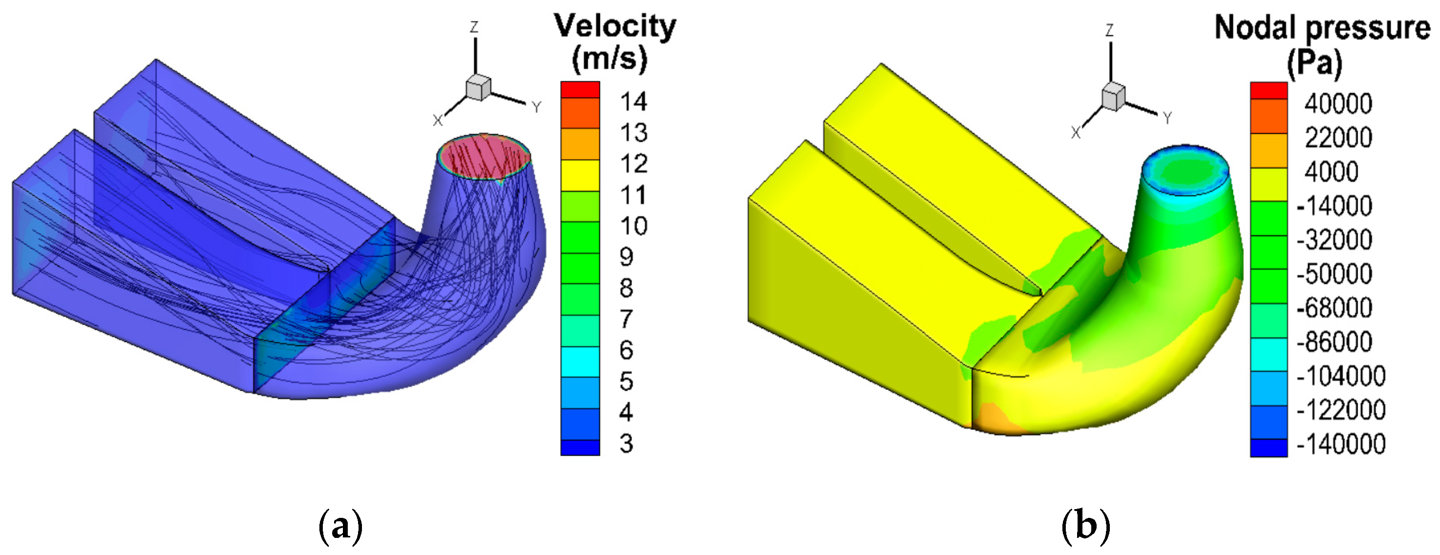
The draft tube is mainly responsible for draining water downstream and recovering partial energy of the flow at the runner outlet, and its type and size can greatly influence the efficiency and stability of the turbine. The flow condition in the elbow section of the draft tube is more complex. Secondary flow may occur when water flows along a vertical straight cone to the elbow and horizontal diffusion section, with nearly 90 degrees turning. At the same time, the diffusing, shrinking, and re-diffusing cross-section of the draft tube along the flow direction may result in uneven distribution of water flow together with local vortices and reflux. Therefore, it is necessary to analyze the flow field and pressure in the draft tube.
The flow condition and pressure contour distribution in the draft tube is illustrated in Figure 9. After flowing through the high-speed rotating runner, the water entered the straight cone section of the draft tube at a higher speed and then decreased gradually along the flow direction. The streamlines inside the draft tube were basically smooth. Higher pressure occurred at the outer side of the elbow, and lower pressure occurred at the inner side. The distribution of velocity and pressure was more uniform in the diffuser section of the draft tube.
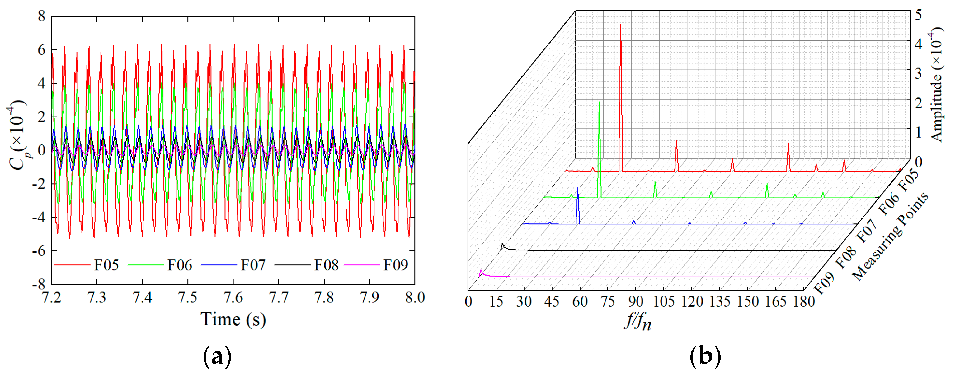
Measuring point F05 was placed at the 0.3 D straight cone section of the draft tube according to the IEC standard. Figure 10 shows the time and frequency domain graph of Cp at the measuring points F05~F09 in the draft tube. The first main frequency of Cp at the measuring points F05, F06, and F07 was 30fn, twice blades passing frequency, which indicated that the pressure fluctuation in the draft tube was greatly affected by periodically rotating blades. Low frequency pressure pulsation existed at the measuring points F08 and F09 near the outlet with merely small amplitude.
3.4. Comparison with the In-Site Data
Three measuring points were chosen and respectively placed at the head cover, vaneless region, and bottom ring to validate the simulation results against the in-site data. Table 1 shows the comparison of the calculated and in-site peak to peak values of the relative pressure pulsations with 97% confidence for different measuring points. The computed ΔH/H was slightly overestimated at the vaneless region, while the relative pressure pulsation at the head cover and bottom ring was slightly lower than the in-site data. Overall, calculated amplitudes of the pulsations agreed well with the in-site data, which provided a reliable basis for analyzing the pressure pulsation transmission path.
4. Pressure Pulsation Transmission Path in the Fluid Flow
Hydraulic vibration is the main vibration source in the hydropower house. The transmission of transient pressure pulsation caused by dynamic interaction between fluid and solid plays a basically important role in the analysis of the structural vibration transmission path in the hydropower house. In this section, the transmission direction of the pressure pulsation was analyzed and the pressure pulsation transmission path in fluid domain was identified, which lays a foundation for investigation into the coupled vibration of the hydropower house.
4.1. Case Study
The transmission direction of the pressure pulsation can be judged by the value of transfer entropy. According to the physical meaning of time-delayed transfer entropy, the transfer entropy in the positive direction of information transmission is larger than that in the negative direction. For a specific combination of two measuring points, if T(i + 1→i) is larger than T(i→i + 1) at most time delays, considering the phase difference between the curves, we can conclude the information transfers from measuring point i + 1 to i.
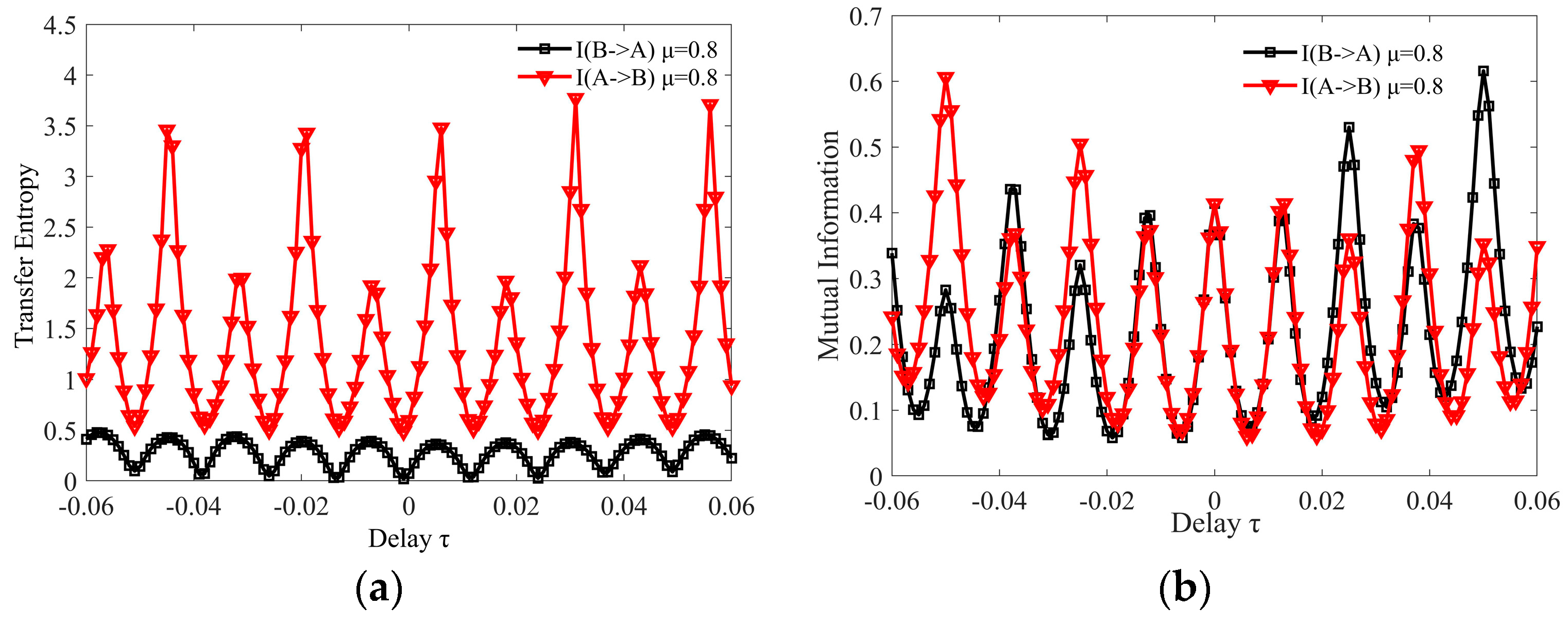
In order to demonstrate the effectiveness of the programming codes of the time-delayed transfer entropy, a case of information transfer identification was performed by reference to [23]. Two sequences A and B were given on the basis of sine and cosine with the description of A = 0.2sin(2πf1t) + cos(2πf2t), B = μA + 0.1cos(2πf1t)cos(2πf2t) − cos(2πf1t). μ was utilized as an index to measure the correlation degree between the two sequences and was given a value of 0.8 to compare the results. It is obviously inferred from the formulas of the two sequences that A is a component of B. Hence, we can test the sensitivity of time-delayed transfer entropy in terms of directivity.
Figure 11 shows the calculation results using time-delayed transfer entropy and the time-delayed mutual information method. It can be intuitively inferred from Figure 11a that the information was transmitted from A to B, which conforms to the actual situation. However, the two curves calculated by the mutual information method overlapped with each other, and the directivity of information transmission cannot be detected. This comparison highlights the superiority of using time-delayed transfer entropy methodology.
4.2. Pulsation Transmission Path Identification Based on Original Data
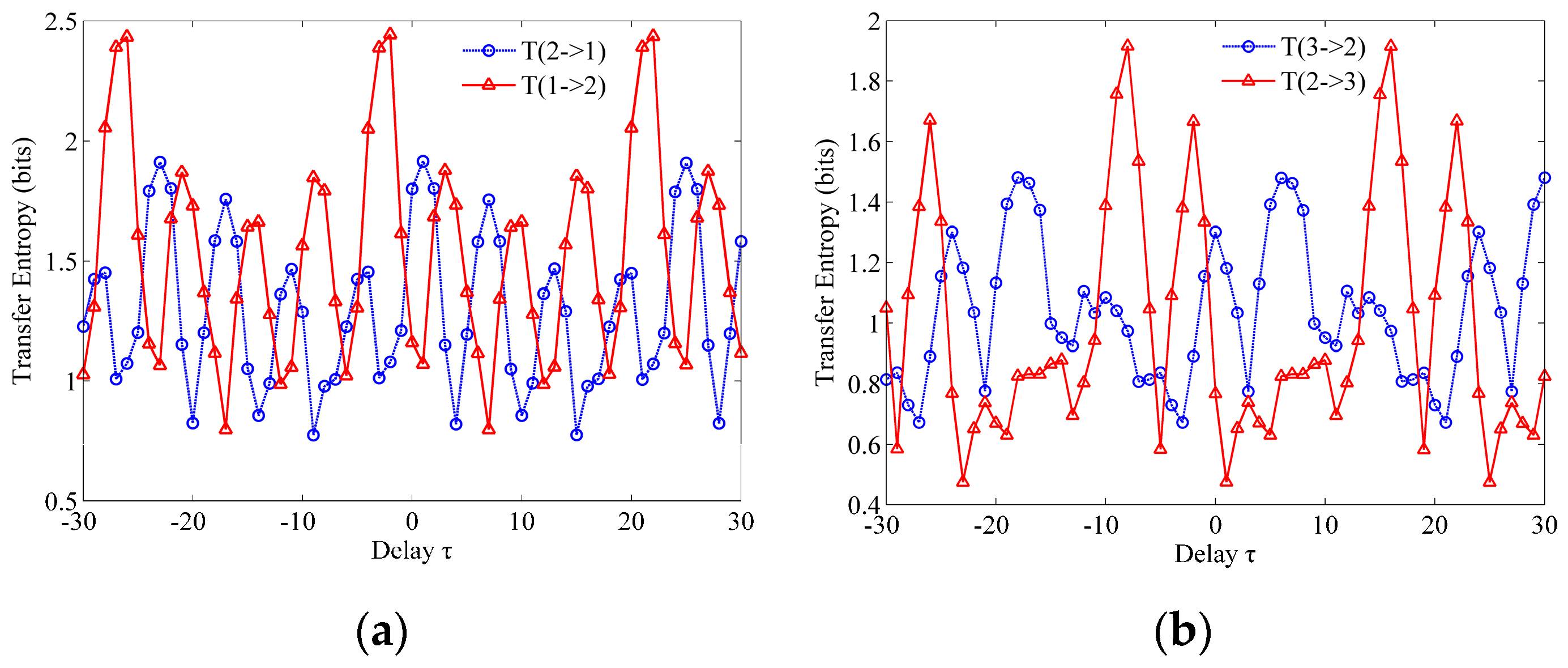
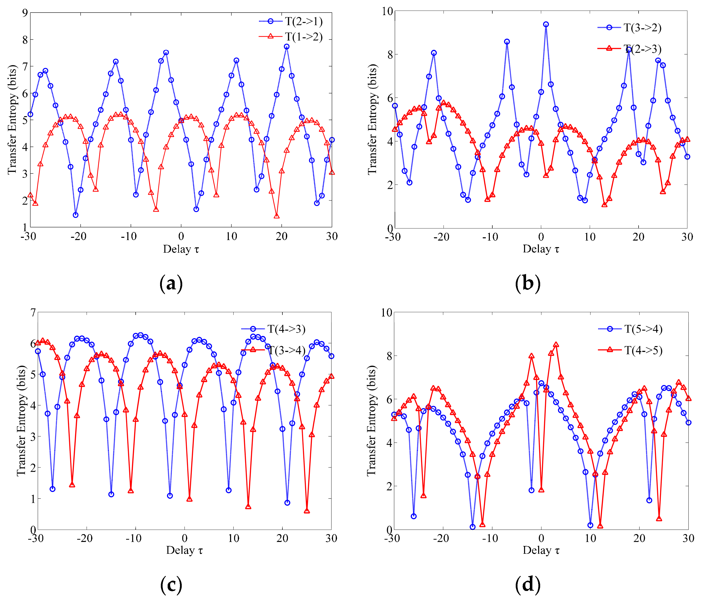
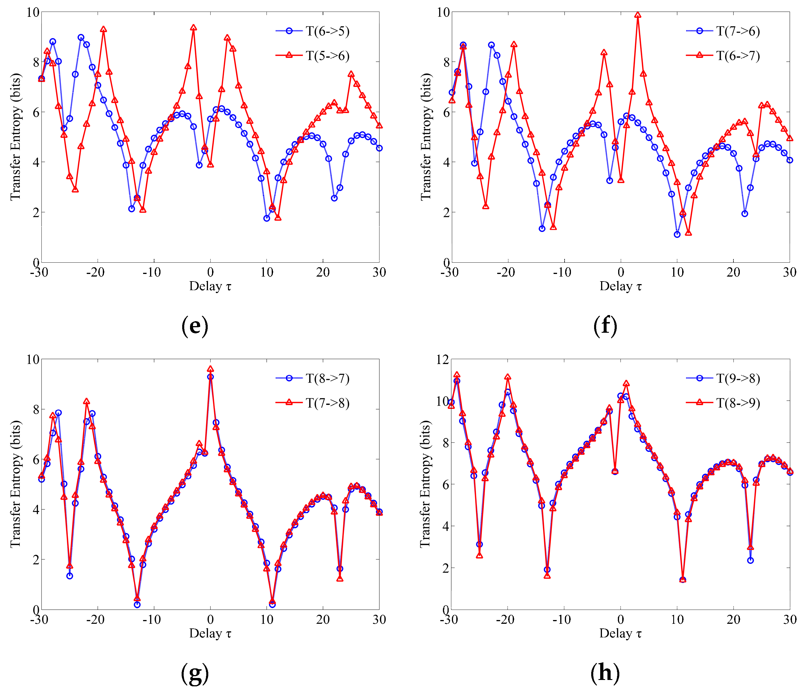
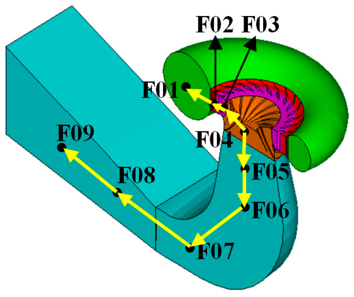
Measuring points were pairwise combined according to the distance between them along the flow direction. Time-varying pressure pulsation of the measuring points in each combination was obtained based on the FSI calculation results under the design operation, and the original nodal pressure data were substituted into Equation (6) to calculate the time-delayed transfer entropy T(i + 1→i) and T(i→i + 1). Figure 12 shows the time-delayed transfer entropy curve of the measuring points. Obviously identified transmission direction of pressure pulsation was as follows: measuring point F04 at the runner → measuring point F03 at the runner inlet, measuring point F05 at the 0.3 D straight cone section of the draft tube → measuring point F06 at the 1.0 D straight cone section of the draft tube → measuring point F07 at the elbow section of the draft tube → measuring point F08 at the diffusion section of the draft tube → measuring point F09 at the diffusion section of the draft tube. The pressure pulsation transmission path is presented in Figure 13.
The calculation results of the time-delayed transfer entropy of measuring points F03 and F04 render obvious different values among the results of all the fluid measuring points, shown in Figure 12c. From the curve, we can see T(4→3) is obviously larger than T(3→4), which indicates a clear transmission direction of pressure pulsation from the runner to the runner inlet. The identified pressure transmission direction is not exactly consistent with the original nodal pressure damping direction, which means the constant static pressure may be irrelevant in identifying the pressure transmission direction using the proposed method. The pressure transmission direction in the draft tube conformed to the actual regularity. After water flowed into the draft tube through a high-speed rotating runner, the pressure pulsation generated in the straight cone section of the draft tube propagated downstream along the flow direction and produced a relatively weak pulsation in the elbow section of the draft tube. The influence of the pressure pulsation in the diffusion section of the draft tube on the flow field in the straight cone and elbow section was small due to the long distance to the vibration source. Therefore, the transmission direction of the pressure pulsation in the draft tube was from the straight cone section to the elbow section, and then to the diffusion section of the draft tube. In fact, the axisymmetric small-disturbance standing waves were generated in the swirling flow of the turbine runner [24], which will propagate both upstream against the flow direction and downstream along the flow direction.
It is noteworthy that the transmission direction between the runner and the straight cone section of the draft tube was not clear, which lay in the complex flow pattern at the runner outlet. When water flowed through the high-speed rotating runner into the draft tube, a vortex would be generated in the draft tube, which caused the fluid pressure pulsation and coupled vibration of the hydropower house. The pressure pulsations caused by the vortex rope in the draft tube interacted with that caused by the rotation of the runner, and the transmission path between the two positions was difficult to identify. In addition, the calculation curves of the time-delayed transfer entropy of adjacent points F01 and F02, and F02 and F03 were overlapped, which made it hard to identify the absolute relationship. This result was associated with the flow direction and the relative position to the runner and also illustrated that the pressure pulsation transmission of the hydraulic vibration source of the hydropower house was the mutual result of multiple transmission signals. Wavelet analysis can be conducted for further identification of the transmission direction of the pressure pulsation.
4.3. Pulsation Transmission Path Identification Based on Wavelet Transform Method
Wavelet theory was adopted to extract the single frequency component of the time-varying pressure of the measuring points to further analyze the transmission regularity. Based on the calculated FFT (fast Fourier transform) results, the characteristic frequency of the pressure pulsation of the measuring points was blades passing frequency 15fn (18.75 Hz) multiple times. Therefore, the time history of the pressure values of a single frequency component 18.75 Hz was extracted from the original calculation data using the wavelet transform method, and then time-delayed transfer entropy was calculated to identify the pulsation transmission direction of the single frequency component between the measuring points.
Figure 14 illustrates the calculation results of the time-delayed transfer entropy of fluid pressure pulsation of characteristic frequency 18.75 Hz for the same measuring points. Stronger transmission directionality was detected between the measuring points compared with the calculation results of the original time-varying pressure data. The recognized pressure transmission path of single frequency f = 18.75 Hz was as follows: measuring point F01 at the spiral casing ← measuring point F02 between the stay vane and guide vane ← measuring point F03 at the runner inlet ← measuring point F04 at the runner → measuring point F05 at the 0.3 D straight cone section of the draft tube → measuring point F06 at the 1.0 D straight cone section of the draft tube → measuring point F07 at the elbow section of the draft tube → measuring point F08 at the diffusion section of the draft tube → measuring point F09 at the diffusion section of the draft tube.
Every curve presented in Figure 14 renders five wave crests and troughs, which may be ascribed to the characteristic frequency 18.75 Hz adopted in the wavelet transform method. Compared to the calculation results of the time-delayed transfer entropy based on original data, the transmission direction between measuring points F01 and F02, and F02 and F03 was more evident to identify based on a combination of the wavelet theory and time-delayed transfer entropy method. However, for the measuring points groups F07 and F08, and F08 and F09, the transmission direction was difficult to distinguish due to the prominent low frequency component at measuring points F08 and F09. Although the influence of the blades passing frequency has been greatly weakened, weak pulsation transmission information can also be identified from Figure 14g,h. The identified pressure pulsation transmission path is shown in Figure 15.
5. Conclusions
This paper established and explored a three-dimensional mechanics–hydraulics–concrete structure coupled numerical model of a Francis hydropower house. Calculation of an unsteady turbulent flow field in the entire flow channel during design operation was carried out using the DES turbulence model and two-way iterative FSI method. Analysis of spatial distribution features of transient velocity, pressure, and streamlines was performed, and time and frequency domain analysis of the pressure pulsation of typical measuring points was conducted. A method for identifying the fluid pressure pulsation transmission path was proposed using the self-programming code in MATLAB software based on the time-delayed transfer entropy method and wavelet theory. The effects of the traditional transfer entropy method and the method proposed in this paper on identifying the fluid pressure pulsation transmission path were studied and compared, and the pressure pulsation transmission law in the entire channel through the Francis turbine was revealed. The proposed methodology was applied to the pulsation transmission analysis of a Francis turbine operating at the BEP in this study. For other types of turbine operating at extreme load ranges, the proposed methodology is also applicable, but the identified results may not always be the same. The main conclusions are as follows:
- (1)
- Unsteady flow features in the spiral casing, vaneless region, and draft tube were analyzed based on FSI calculation in design operation. The velocity and pressure in the spiral casing and vaneless region rendered symmetrical distribution in the circumference. Pressure gradually decreased with the increasing velocity as water flowed into the high-speed rotating runner. Smaller velocity and higher pressure occurred at the outer side of the elbow, and larger velocity and lower pressure occurred at the inner side. In the diffuser section of the draft tube, distribution of velocity and pressure was more uniform. The overall pressure transition was smooth without obvious sudden changes, and the streamline distribution was continuous. Frequency analysis of the pressure of the measuring points showed that the first main frequency was the multiple times blades passing frequency, so the main hydraulic vibration source was the blades’ rotation.
- (2)
- The transmission path of the pressure pulsation in the flow channel was identified based on the time-delayed transfer entropy and wavelet transform method using MATLAB software. The pressure pulsation in the components downstream the high-speed rotating runner propagated along the flow direction, which was clear and easy to identify using time-delayed transfer entropy. For the fluid flow upstream the turbine, the pressure transmission path was more complicated to identify, since the pressure propagated against the flow direction. The wavelet transform method was used to extract the time-varying pressure in terms of the characteristic frequency, and the pressure pulsation transmission law was obtained in which the axisymmetric small-disturbance standing waves transmitted from runner to upstream and downstream, respectively, which illustrates the type of draft tube and the connection with the runner are critical to the design of the hydraulic turbine, as well as verifying the rationality of using time-delayed transfer entropy and the wavelet transform method to identify the transmission path.
In summary, it is flexible and practical to use time-delayed transfer entropy for identification of the pressure pulsation transmission path, which provides a novel idea for analyzing the hydraulic vibration transmission path in the structure of the hydropower house and lays a firm basis for exploring the coupled vibration of the unsteady flow and hydropower house. However, this research mainly focused on the operation of Francis turbine at the BEP. Extreme load ranges such as part load condition and transient load variations during operations of the Francis turbine are more relevant for actual requirements in the energy market and will be our future focus.
Author Contributions
Conceptualization, S.W., L.Z., and G.Y.; Data curation, S.W. and G.Y.; Formal analysis, S.W. and G.Y.; Funding acquisition, S.W., L.Z., and C.G.; Investigation, S.W. and G.Y.; Supervision, L.Z.; Validation, S.W. and G.Y.; Writing—original draft, S.W.; Writing—review and editing, S.W., L.Z., and G.Y.
Funding
This work was financially supported by the National Key Research and Development Plan of China (Grant No. 2017YFC0404903), the Fundamental Research Funds for the Central Universities (Grant No. 2016B41014).
Conflicts of Interest
The authors declare no conflict of interest.
References
- Trivedi, C.; Cervantes, J.M.; Dahlhaug, G.O. Experimental and Numerical Studies of a High-Head Francis Turbine: A Review of the Francis-99 Test Case. Energies 2016, 9, 74. [Google Scholar] [CrossRef]
- Arispe, T.M.; Oliveira, W.D.; Ramirez, R.G. Francis turbine draft tube parameterization and analysis of performance characteristics using CFD techniques. Renew. Energy 2018, 127, 114–124. [Google Scholar] [CrossRef]
- Trivedi, C.; Gogstad, P.J.; Dahlhaug, O.G. Investigation of the unsteady pressure pulsations in the prototype Francis turbines—Part 1: Steady state operating conditions. Mech. Syst. Signal Process. 2018, 108, 188–202. [Google Scholar] [CrossRef]
- Li, D.; Sun, Y.; Zuo, Z.; Liu, S.; Wang, H.; Li, Z. Analysis of Pressure Fluctuations in a Prototype Pump-Turbine with Different Numbers of Runner Blades in Turbine Mode. Energies 2018, 11, 1474. [Google Scholar] [CrossRef]
- Mössinger, P.; Jesterzürker, R.; Jung, A. In Francis-99: Transient CFD simulation of load changes and turbine shutdown in a model sized high-head Francis turbine. J. Phys. Conf. Ser. 2017, 782, 012001. [Google Scholar] [CrossRef]
- Chalghoum, I.; Elaoud, S.; Akrout, M.; Taieb, E.H. Transient behavior of a centrifugal pump during starting period. Appl. Acoust. 2016, 109, 82–89. [Google Scholar] [CrossRef]
- Goyal, R.; Trivedi, C.; Gandhi, B.K.; Cervantes, M.J. Numerical Simulation and Validation of a High Head Model Francis Turbine at Part Load Operating Condition. J. Inst. Eng. 2017, 99, 557–570. [Google Scholar] [CrossRef]
- Xiao, R.; Wang, Z.; Luo, Y. Dynamic Stresses in a Francis Turbine Runner Based on Fluid-Structure Interaction Analysis. Tsinghua Sci. Technol. 2008, 13, 587–592. [Google Scholar] [CrossRef]
- Dompierre, F.; Sabourin, M. Determination of turbine runner dynamic behaviour under operating condition by a two-way staggered fluid-structureinteraction method. IOP Conf. Ser. Earth Environ. Sci. 2010, 12, 012085. [Google Scholar] [CrossRef]
- Overbey, L.A.; Todd, M.D. Effects of noise on transfer entropy estimation for damage detection. Mech. Syst. Signal Process. 2009, 23, 2178–2191. [Google Scholar] [CrossRef]
- Liu, G.H.; Xie, Z.K. A modified transfer entropy method for damage detection of beam structures. Zhejiang Daxue Xuebao (Gongxue Ban)/J. Zhejiang Univ. 2014, 27, 136–144. [Google Scholar]
- Minakov, A.V.; Platonov, D.V.; Dekterev, A.A.; Sentyabov, A.V.; Zakharov, A.V. The analysis of unsteady flow structure and low frequency pressure pulsations in the high-head Francis turbines. Int. J. Heat Fluid Flow 2015, 53, 183–194. [Google Scholar] [CrossRef]
- Gavrilov, A.; Dekterev, A.; Minakov, A.; Platonov, D.; Sentyabov, A. Application of hybrid methods to calculations of vortex precession in swirling flows. In Progress in Hybrid RANS-LES Modelling; Springer: Berlin/Heidelberg, Germany, 2012; pp. 449–459. [Google Scholar]
- Spalart, P.; Allmaras, S. A one-equation turbulence model for aerodynamic flows. In Proceedings of the 30th Aerospace Sciences Meeting and Exhibit, Reno, NV, USA, 6–9 January 1992; p. 439. [Google Scholar]
- Guo, Y.; Kato, C. Investigation of the Performance of DES-SA Model in Several Turbulent Flows. Seisan Kenkyu 2008, 60, 75–80. [Google Scholar]
- Tu, S.; Shahrouz, A.; Reena, P.; Marvin, W. An implementation of the Spalart-Allmaras DES model in an implicit unstructured hybrid finite volume/element solver for incompressible turbulent flow. Int. J. Numer. Methods Fluids 2010, 59, 1051–1062. [Google Scholar] [CrossRef]
- Wei, S.; Zhang, L. Vibration analysis of hydropower house based on fluid-structure coupling numerical method. Water Sci. Eng. 2010, 3, 75–84. [Google Scholar]
- Nichols, J.M.; Seaver, M.; Trickey, S.T. A method for detecting damage-induced nonlinearities in structures using information theory. J. Sound Vib. 2006, 297, 1–16. [Google Scholar] [CrossRef]
- Overbey, L.A.; Todd, M.D. Dynamic system change detection using a modification of the transfer entropy. J. Sound Vib. 2009, 322, 438–453. [Google Scholar] [CrossRef]
- Schreiber, T. Measuring information transfer. Phys. Rev. Lett. 2000, 85, 461–464. [Google Scholar] [CrossRef]
- Nichols, J.M. Examining structural dynamics using information flow. Probabilistic Eng. Mech. 2006, 21, 420–433. [Google Scholar] [CrossRef]
- Nichols, J.; Seaver, M.; Trickey, S.; Todd, M.; Olson, C.; Overbey, L. Detecting nonlinearity in structural systems using the transfer entropy. Phys. Rev. E 2005, 72, 046217. [Google Scholar] [CrossRef]
- Wang, H.; Wang, N.; Lian, J. Vibration transfer path identification of the hydropower house based on transfer entropy. J. Hydraul. Eng. 2018, 49, 732–740. [Google Scholar]
- Susan-Resiga, R.; Ciocan, G.D.; Anton, I.; Avellan, F. Analysis of the Swirling Flow Downstream a Francis Turbine Runner. J. Fluids Eng. 2006, 128, 177–189. [Google Scholar] [CrossRef]
Figure 1.
Computational domain. (a) Fluid–structure interaction (FSI) model, (b) fluid model.

Figure 2.
3D structured grids for the fluid domain. (a) Spiral casing, (b) stay and guide vane, (c) runner, (d) draft tube.
Figure 2.
3D structured grids for the fluid domain. (a) Spiral casing, (b) stay and guide vane, (c) runner, (d) draft tube.

Figure 3.
Cross-section diagram and 3D structured grids for the solid domain. (a) River-along section diagram, (b) 3D structured grids.
Figure 3.
Cross-section diagram and 3D structured grids for the solid domain. (a) River-along section diagram, (b) 3D structured grids.

Figure 4.
Measuring points distribution in the fluid flow region during numerical calculation process. (a) Top view section diagram, (b) river-along section diagram.
Figure 4.
Measuring points distribution in the fluid flow region during numerical calculation process. (a) Top view section diagram, (b) river-along section diagram.

Figure 5.
Distribution of velocity, streamline, and pressure in the spiral casing and vaneless region. (a) Velocity and streamlines distribution, (b) pressure contour.
Figure 5.
Distribution of velocity, streamline, and pressure in the spiral casing and vaneless region. (a) Velocity and streamlines distribution, (b) pressure contour.

Figure 6.
Time and frequency analysis of Cp at the measuring points F01~F03. (a) Time domain graph, (b) frequency domain graph.
Figure 6.
Time and frequency analysis of Cp at the measuring points F01~F03. (a) Time domain graph, (b) frequency domain graph.

Figure 7.
Velocity and pressure distribution in the runner. (a) Velocity contour, (b) pressure contour.
Figure 7.
Velocity and pressure distribution in the runner. (a) Velocity contour, (b) pressure contour.

Figure 8.
Time and frequency analysis of Cp at the measuring point F04. (a) Time domain graph, (b) frequency domain graph.
Figure 8.
Time and frequency analysis of Cp at the measuring point F04. (a) Time domain graph, (b) frequency domain graph.

Figure 9.
Distribution of velocity, streamline, and pressure in the draft tube. (a) Velocity and streamlines distribution, (b) pressure contour.
Figure 9.
Distribution of velocity, streamline, and pressure in the draft tube. (a) Velocity and streamlines distribution, (b) pressure contour.

Figure 10.
Time and frequency analysis of Cp at the measuring points F05~F09. (a) Time domain graph, (b) frequency domain graph.
Figure 10.
Time and frequency analysis of Cp at the measuring points F05~F09. (a) Time domain graph, (b) frequency domain graph.

Figure 11.
Comparison of results between transfer entropy and the mutual information method. (a) Result using the transfer entropy method, (b) result using the mutual information method.
Figure 11.
Comparison of results between transfer entropy and the mutual information method. (a) Result using the transfer entropy method, (b) result using the mutual information method.

Figure 12.
Time-delayed transfer entropy curve of the original fluid pressure pulsation. Transfer entropy between measuring points F01 and F02 (a), F02 and F03 (b), F03 and F04 (c), F04 and F05 (d), F05 and F06 (e), F06 and F07 (f), F07 and F08 (g), and F08 and F09 (h).
Figure 12.
Time-delayed transfer entropy curve of the original fluid pressure pulsation. Transfer entropy between measuring points F01 and F02 (a), F02 and F03 (b), F03 and F04 (c), F04 and F05 (d), F05 and F06 (e), F06 and F07 (f), F07 and F08 (g), and F08 and F09 (h).


Figure 13.
Presentation of pressure pulsation transmission path based on the original fluid pressure pulsation.
Figure 13.
Presentation of pressure pulsation transmission path based on the original fluid pressure pulsation.

Figure 14.
Time-delayed transfer entropy curve of the frequency of 18.75 Hz fluid pressure pulsation. Transfer entropy between measuring points F01 and F02 (a), F02 and F03 (b), F03 and F04 (c), F04 and F05 (d), F05 and F06 (e), F06 and F07 (f), F07 and F08 (g), and F08 and F09 (h).
Figure 14.
Time-delayed transfer entropy curve of the frequency of 18.75 Hz fluid pressure pulsation. Transfer entropy between measuring points F01 and F02 (a), F02 and F03 (b), F03 and F04 (c), F04 and F05 (d), F05 and F06 (e), F06 and F07 (f), F07 and F08 (g), and F08 and F09 (h).


Figure 15.
Presentation of pressure pulsation transmission path based on the 18.75 Hz wavelet transformation.
Figure 15.
Presentation of pressure pulsation transmission path based on the 18.75 Hz wavelet transformation.


Table 1.
ΔH/H with 97% confidence at different positions for simulation and in-site data.
| Location | ΔH/H with 97% Degree of Confidence (%) | Error (%) | |
|---|---|---|---|
| Simulation Results | In-Site Data | ||
| Head cover | 0.26 | 0.31 | 16 |
| Vaneless region | 0.85 | 0.82 | 4 |
| Bottom ring | 0.40 | 0.41 | 2 |
© 2019 by the authors. Licensee MDPI, Basel, Switzerland. This article is an open access article distributed under the terms and conditions of the Creative Commons Attribution (CC BY) license (http://creativecommons.org/licenses/by/4.0/).
Share and Cite
MDPI and ACS Style
Wang, S.; Zhang, L.; Yin, G.; Guan, C. Research on Unsteady Hydraulic Features of a Francis Turbine and a Novel Method for Identifying Pressure Pulsation Transmission Path. Water 2019, 11, 1216. https://doi.org/10.3390/w11061216
AMA Style
Wang S, Zhang L, Yin G, Guan C. Research on Unsteady Hydraulic Features of a Francis Turbine and a Novel Method for Identifying Pressure Pulsation Transmission Path. Water. 2019; 11(6):1216. https://doi.org/10.3390/w11061216
Chicago/Turabian StyleWang, Shuo, Liaojun Zhang, Guojiang Yin, and Chaonian Guan. 2019. "Research on Unsteady Hydraulic Features of a Francis Turbine and a Novel Method for Identifying Pressure Pulsation Transmission Path" Water 11, no. 6: 1216. https://doi.org/10.3390/w11061216
Note that from the first issue of 2016, this journal uses article numbers instead of page numbers. See further details here.