Forcing the Penman-Montheith Formulation with Humidity, Radiation, and Wind Speed Taken from Reanalyses, for Hydrologic Modeling


Department of Civil and Water Engineering, Laval University, Québec, QC G1V 0A6, Canada
*
Author to whom correspondence should be addressed.
Water 2019, 11(6), 1214; https://doi.org/10.3390/w11061214
Submission received: 8 April 2019
/
Revised: 27 May 2019
/
Accepted: 3 June 2019
/
Published: 11 June 2019
(This article belongs to the Section Hydrology)
Abstract
:The Penman-Monteith reference evapotranspiration (ET0) formulation was forced with humidity, radiation, and wind speed (HRW) fields simulated by four reanalyses in order to simulate hydrologic processes over six mid-sized nivo-pluvial watersheds in southern Quebec, Canada. The resulting simulated hydrologic response is comparable to an empirical ET0 formulation based exclusively on air temperature. However, Penman-Montheith provides a sounder representation of the existing relations between evapotranspiration fluctuations and climate drivers. Correcting HRW fields significantly improves the hydrologic bias over the pluvial period (June to November). The latter did not translate into an increase of the hydrologic performance according to the Kling-Gupta Efficiency (KGE) metric. The suggested approach allows for the implementation of physically-based ET0 formulations where HRW observations are insufficient for the calibration and validation of hydrologic models and a potential reinforcement of the confidence affecting the projection of low flow regimes and water availability.
Keywords:
hydrology; modeling; evapotranspiration; reanalysis; Penman-Monteith; humidity; radiation; wind speed1. Introduction
Evapotranspiration (ET) is a key process in the representation of hydroclimatic flows and budgets. It is defined as the transfer of water vapor to the atmosphere from a surface or through plant stomata. Four main meteorological drivers determine ET fluctuations: air temperature, net radiation, humidity, and wind speed. The ET fluxes are rarely measured, and estimation approaches are affected by large uncertainties. In hydrologic modeling, ET is typically treated as a component of the water balance at the scale of a watershed. Reference evapotranspiration (ET0) is estimated from available climate variables and leads to ET when considering soil water and vegetation cover conditions. Hydrologic models are sensitive to the selection of a given ET0 formulation [1] since it influences their parametric configuration and consequently the yearlong hydrologic regime, including streamflow, soil water content, and snow water equivalent. This influence persists in projections forced under different radiative forcing scenarios [2]. The arguments for deciding upon which ET0 formulation to use are not widely consensual [3,4,5]. On the one hand, empirical ET0 formulations, based exclusively on air temperature, are widely used in hydrology because they are simple to evaluate and perform well in the scope of simulating river flows [6]. On the other hand, formulations integrating to various degrees air humidity, radiation, and wind speed (hereinafter referred to as HRW fields) remains limited by the amount, quality, and representativeness of the available observations.
Forcing hydrologic models with fields simulated by climate reanalyses is becoming progressively common in order to overcome the low density of meteorological observations. Works described in the recent literature [7,8,9,10,11,12,13] demonstrate the capacity of reanalyses to provide consistent hydrologic responses. They may even surpass observations in some instances [9]. The quality of the resulting hydrologic response seems however strongly related to the reanalysis ability to simulate precipitation [8,14]. Downscaling simulated precipitation and correcting bias may substantially improve simulated flows, especially for watersheds presenting complex topographic features [12]. Forcing hydrologic models with reanalyses is typically limited to the use of precipitation and temperature fields and, therefore, to empirical ET0 formulations based exclusively on air temperature.
The ability of reanalyses to simulate HRW fields and their relevance to hydrologic modeling is much less documented [15,16,17]. The correspondence between ET0 values from the Penman-Montheith (PM) formulation respectively forced by in situ observations and fields taken from a reanalysis have been demonstrated over China with the European Centre for Medium-Range Weather Forecasting (ECMWF) ERA-Interim reanalysis [18] and over the Iberian Peninsula with the National Center for Environmental Prediction/National Center for Atmospheric Research(NCEP/NCAR) reanalysis [19]. Huang et al. [20] combined surface radiation and temperature from the National Aeronautics and Space Administration–Clouds and the Earth’s Radiant Energy System (NASA-CERES) and surface specific humidity from the NASA-Modern Era Retrospective-analysis for Research and Applications (MERRA) reanalysis to force the maximum-entropy-production (MEP) model of surface heat fluxes. Yao et al. [21] estimate ET0 by forcing the PM formulation with a combination of the Global Energy and Water Cycle Experiment (GEWEX) Surface Radiation Budget dataset (SRB) and weather observations. The authors conclude that a PM-based approach provides consistent interannual trajectories relative to water budget estimates.
Sperna Weiland et al. [22] forced six ET0 formulations on a global scale with the NCEP Climate Forecast System Reanalysis (CFSR) and CRU dataset (Climate Research Unit, University of East Anglia) and concluded that PM does not outperform simpler ET0 formulations. They argued that their finding may be explained by the limited capacity of the source data, CRU and CFSR, to reproduce the atmospheric fields that forces the PM formulation. Jones et al. [23] demonstrated the benefit of correcting biases in ERA-Interim HRW fields. Sen Gupta and Tarboton [24] developed and applied a downscaling method for temperature, relative humidity, radiation and wind speed taken from MERRA reanalysis in order to simulate the snowpack at 173 sites across the United States. None of the above focused on the hydrologic response at the watershed scale. Essou et al. [25] combined precipitation and temperature observations with supplemental fields from ERA-Interim, CFSR, and MERRA reanalyses for hydrologic modeling. They compared the weighted-average of the meteorological sources and of the hydrologic response. They found that both methods improve the hydrologic response of a large number of watersheds spread across the United States and Canada. Lauri et al. [11] demonstrated the interest of combining temperature simulated by CFSR with precipitation observation for simulating the Mekong streamflow.
The work described in this study aims to answer the following question: are humidity, radiation, and wind speed (HRW fields), as simulated by reanalyses, functional surrogates to observations in providing a consistent, physically-based, simulated hydrologic response. The Penman-Montheith formulation is forced by a combination of interpolated temperature and precipitation observations and HRW fields taken from four state-of-the-art reanalyses. The resulting hydrologic responses (simulated streamflow and state variables, here focusing on evapotranspiration) are evaluated and compared to a temperature-based ET0 formulation. The study also evaluates the impact of reanalyses biases on the simulated hydrologic response and explores a calibration-based (observation-free) correction of the forcing HRW fields.
The suggested approach allows a pragmatic solution to simulate hydrologic processes over a watershed using a more physically-based ET0 formulation even where HRW observations are insufficient or absent. Without formally exploring this idea, Auerbach et al. [7] suggested exploiting the HRW fields from the CFSR reanalysis in order to simulate hydrologic processes on more mechanistic grounds. Considering the climate change-driven increase of the air temperature and modification of the HRW fields, we believe the usage of a physically-based ET0 formulation, even partially forced by reanalyses, supports the construction of more reliable streamflow projections at the catchment scale.
2. Domain, Data, and Methodology
2.1. Domain
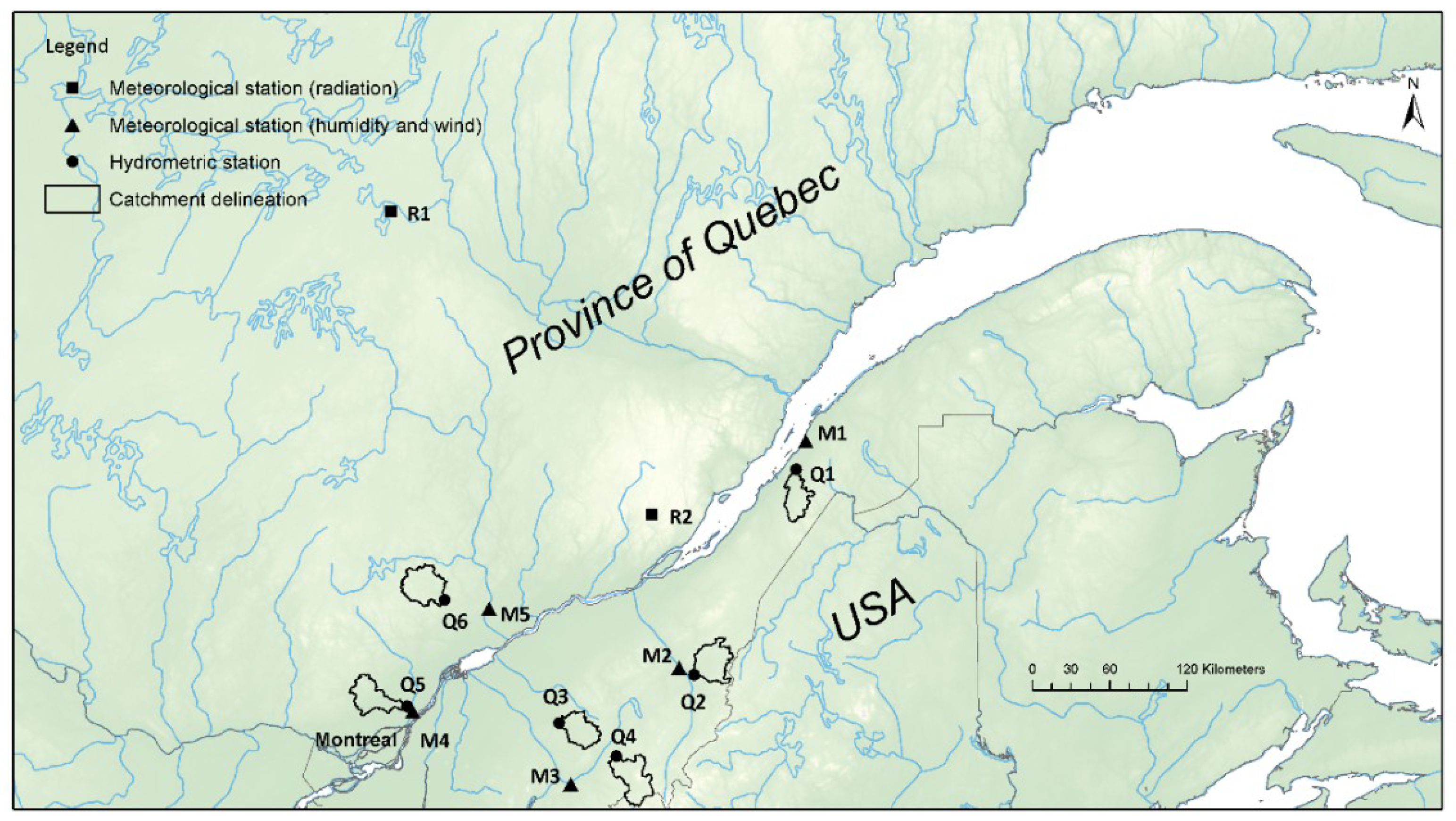
The analysis is conducted over six intermediate-size catchments (512 to 761 km2) located in the Province of Quebec, Canada, between latitudes 45° N and 48° N and longitudes −69° E and −75° E (Q1 to Q6, Figure 1). Monthly air temperature fluctuates from −13 °C (January) to 20 °C (July) and yearly precipitation, from 1000 mm to 1200 mm. Daily relative humidity remains somehow constant throughout summer and fall (~80%) but declines in April and May (~60%). Daily downwelling shortwave radiation (site R1) peaks in June (5500 W/m2) and plummets in December (1000 W/m2). Daily wind speed is fairly constant from November to March (up to 3 m/s) but lowers throughout summer (2 m/s). All sites are categorized as mixed nivo-pluvial hydrologic regime characterized by an important spring freshet and autumnal highs. Streamflow typically peaks in April when the snowpack melts. A second but lesser peak follows lower autumnal evapotranspiration and intensification of synoptic precipitations. Low flows dominate winter and are common in summer because of the accumulation of the snowfall and of maximum evapotranspiration, respectively. All basins are characterized by moderate slopes (4.1%–13.4%). Forest is the dominant land use (59%–83%) while sites Q3 and Q5 present a significant portion of agricultural and urbanized lands (32% and 35%, respectively). All flows are quite free from the upstream influence of the dam operations, with DOR values (“degree of regulation”) not exceeding 8% for all basins [26].
2.2. Data
Daily hydrometric observations are provided by the Quebec hydrometric network and daily precipitation and temperature observations, from Quebec Climate Monitoring Program. Precipitation and temperature observations are interpolated by kriging on a 0.1-degree grid. Relative humidity and wind speed observations are extracted from the closest Environment and Climate Change Canada weather stations (sites M1 to M5, Figure 1, Table 1). The distance to the corresponding hydrometric station ranges from 6.4 to 49.2 km. Short wave radiation and latent heat flux observations are extracted respectively at Black Spruce/Jack Pine site (R1, 49.27° N and −74.04° E) and Forêt Montmorency (R2, 47.27° N and −71.12° E) experimental sites. R1 is located further north, the distance to sites Q1 to Q6 varies from 304 to 458 km. Data are available from 2005 to 2009 at site R1 and from 2016 to 2018 at site R2.
Preprocessing is applied to the relative humidity, downwelling shortwave radiation, and wind speed (the HRW fields) taken from CFSR [27], MERRA-2 [28], ERA-Interim [29], and the Japanese 55-year atmospheric reanalysis (JRA-55 [30,31]) reanalyses. Experimenting numerous forcing data sets allows the evaluation of the sensitivity of the simulated hydrological response to reanalyses biases. Simulated HRW fields are combined to precipitation and temperature observations for two reasons. First, to circumvent the documented impact of large biases affecting precipitation taken from reanalyses on the simulated hydrological response (see Introduction). Second, precipitation and temperature observations are readily available at the regional scale to force hydrological models on numerous catchments, which is rarely the case for HRW fields. Reanalyses data units are harmonized and integrated into a daily time step. The average daily wind speed is the vector average of the North-South and East-West components. MERRA-2 and JRA-55 relative humidity values are calculated from the air and dew point temperatures using the following formulation:
where RH is the relative humidity (%), Tdw, dew point temperature (°C), T, air temperature (°C), m (–) and Tn (°C), empirical constants for specific temperature ranges.
2.3. Hydrologic Modeling Setup
Table 2 summarizes the hydrologic modeling setup designed for this study. The Richards-9.02.00 version of the physically-based distributed hydrologic model WaSim-ETH [32,33,34] is implemented over the six catchments described in Section 2.1. The river network is generated from a burned 50-m resolution digital elevation model, resampled to 500 m and manually corrected for each catchment. Land use is extracted from various sources provided by local agencies. Reference evapotranspiration (ET0) is evaluated on the Penman-Montheith (PM) formulation [35]:
where λ is the latent vaporization heat (KJ∙Kg−1), E, the latent heat flux (Kg∙m−2), Rn, net radiation (Wh∙m−2), G, soil heat flux (Wh∙m−2), (es − ea), vapour pressure deficit of the air (hPa), ρa, mean air density at constant pressure (Kg∙m−3), cp, specific heat of the air (KJ∙(Kg∙K)−1), Δ, tangent of the saturated vapor pressure curve (hPa∙K−1), γ, psychrometric constant (hPa∙K−1), rs and ra, surface and aerodynamic resistances (s∙m−1).
The PM formulation is forced by observed temperature and humidity, radiation, and wind speed time series taken from reanalyses (Section 2.2) and compared in Section 3.2 and Section 3.3 to the Hamon empirical temperature-based formulation:
where fi is an empirical correction factor (-), hd, day length (h), and es, the saturation vapor pressure at temperature T (hPa).
Solid precipitations are corrected according to Equation (4) using a threshold temperature:
where Pcor is the corrected solid precipitation (mm), as, a correction parameter (-), and Ttr, a threshold temperature for snow/rain transition (°C).
Snowmelt is simulated using a temperature-index degree-day method:
where M is the melting rate (mm∙day−1), c0, a temperature dependent melt factor (mm∙°C−1∙day−1), Tm, the temperature limit for snow melt (°C), and Δt, the simulation time step (24 h).
Vertical fluxes within the unsaturated zone are based on the Richards equation applied to a 10-m deep column composed of 30 numeric layers. An empirical fraction determines the portion of snow melt taken as surface runoff, considering sufficient snow cover on the ground:
where Qs is the surface runoff (mm), Qsnw, snow melt (mm), and QDsnw, a fraction of Qs on Qsnw (-).
Soil textures (percentages of clay, silt, and sand) originate from Shangguan et al. [36], while transient soil hydraulic properties follow Van Genuchten equations. Interflow is generated at soil layer boundaries considering slope and hydraulic conductivity:
where Qh is the interflow (ms−1), ks, the saturated hydraulic conductivity (ms−1), θm, the soil water content in layer m (-), Δz, layer thickness (m), dr, a scaling parameter to consider river density (m−1), and β, the local slope angle (°).
Both surface runoff and interflow are delayed using recession constants:
where Qs,i and Qh,i are delayed surface runoff and interflow at time step i (mm), Qs and Qh, surface runoff and interflow at time step i (mm), Δt, time step (h), ks and kh, recession constants (h).
Table 2 also identifies WaSim-ETH’s free-parameters and the associated ranges of values assigned for calibration. Concordance of available data allows simulation over 31 years, from 1979 to 2009. Calibration is performed from 1980 to 1989 and validation, from 1990 to 2009. Each simulation is allowed an additional year for burning the model. The Pareto archived dynamically dimensioned search (PA-DDS, [37]) is used with 500 iterations to identify optimal parameter sets. A seasonal variant of Kling-Gupta-Efficiency criteria (KGE, [38]) acts as the multi-criteria objective function (OF):
where DJFMAM refers to the period from December to May and JJASON, June to November, r, the correlation coefficient between the observed and simulated values, α, the ratio between the standard deviations, and β, the bias. All components, including KGE, target 1 as the best score.
2.4. Correction of Simulated HRW Fields
In order to improve hydrologic performance, a calibration-based correction is applied to the simulated HRW fields such as:
where are seasonal correction factors (DJFMAM vs. JJASON, additive for H and multiplicative for R and W), H′, R′ and W′, corrected fields.
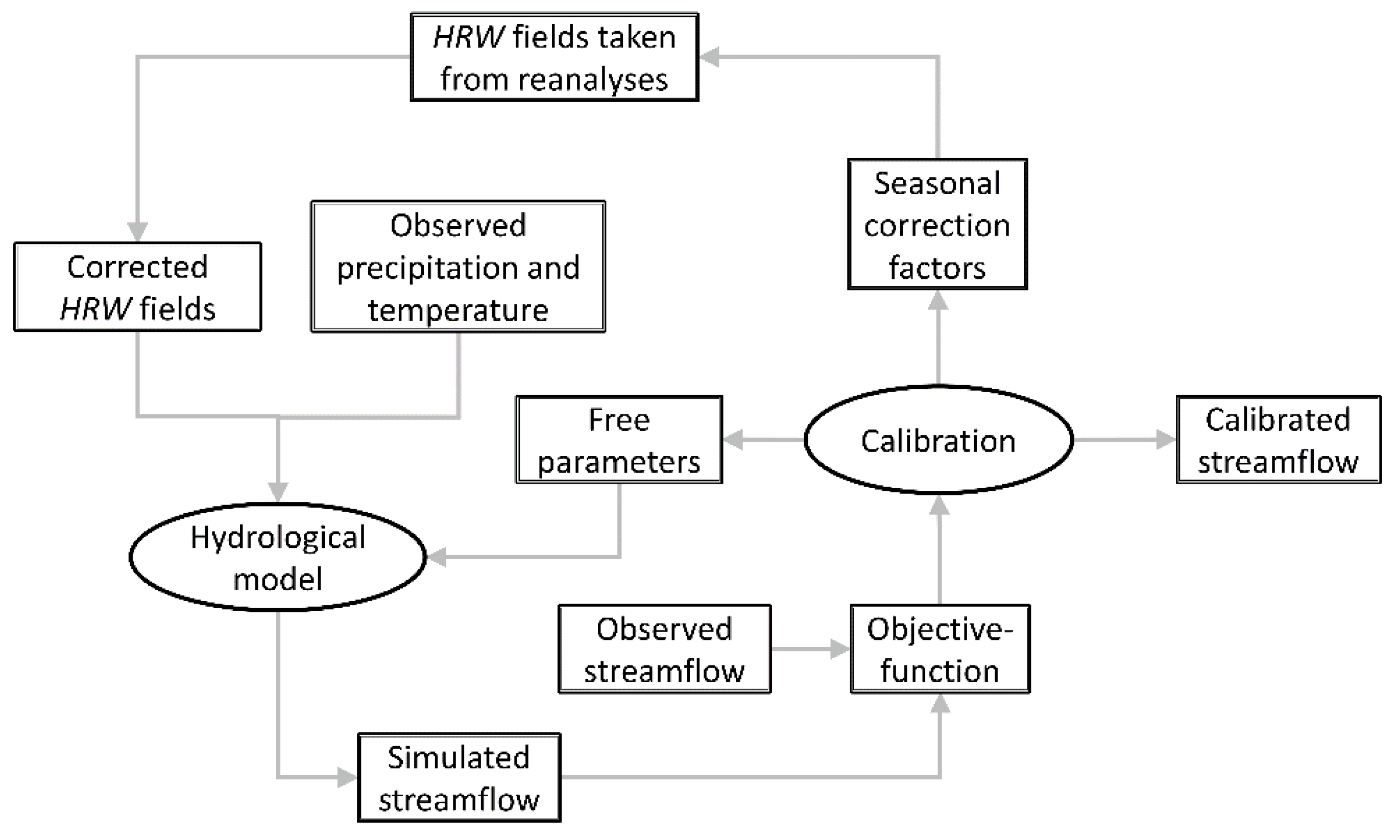
Figure 2 details the calibration of the seasonal correction factors concomitantly to the free-parameters of the hydrologic model. Random initial values are used. Correction is applied to the HRW fields as prescribed by Equations (12) to (14). Corrected HRW fields are combined to observed precipitations and temperature in order to force the hydrologic model simulating streamflow. The multi-criteria objective function (Equation (10)) is computed from simulated and observed streamflow values. Calibration converges iteratively toward an optimal solution producing the final calibrated streamflow. Boundaries constraining optimized values of correction factors are here fixed at [−15%;+15%] for relative humidity and [0.75;1.25] for radiation and wind speed. Corrected relative humidity is post-processed to be bounded between 0 and 1.
3. Results
3.1. Meteorological Performance Values
Table 3 presents the meteorological performance values of CFSR, MERRA-2, ERA-Interim, and JRA-55 simulation of the humidity, radiation, and wind speed observations, while mean (M) and range (R) values synthetize the performance across all four reanalyses. Performance is expressed as KGE and its α, β and r components (Equation (11)) are evaluated from June to November between stations M1 to M5 and R1 and simulated data at the nearest grid points. All four reanalyses are more successful at simulating radiation than humidity and wind speed. Radiation performance values are mainly driven by their correlation and variance components. Humidity offers weaker correlations but good biases. Wind speed performance is less uniform in terms of bias and variance. It provides, however, relatively accurate correlations. Overall, HRW fields are quite comparable from one reanalysis to another. JRA-55 is better simulating humidity (KGEJRA,H = 0.70) and MERRA-2, wind speed (KGEMRA,W = 0.63). On the other hand, CFSR is less precise simulating radiation (KGECFS,R = 0.84).
3.2. Hydrologic Performance Values
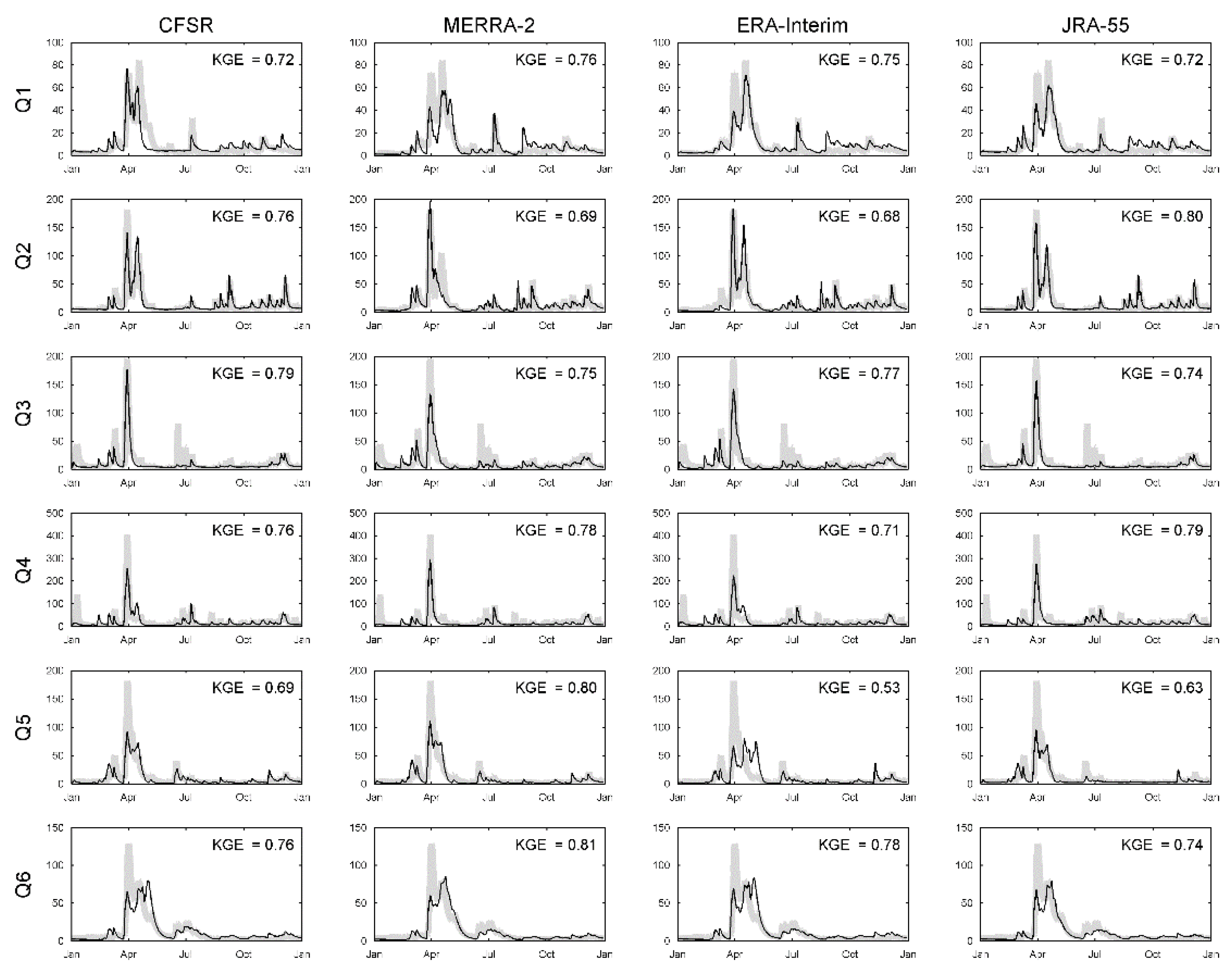
Figure 3 presents 2008 (validation) hydrographs for the raw HRW fields at sites Q1 to Q6 (Figure 1) and for CFSR, MERRA-2, ERA-Interim, and JRA-55 reanalyses. Annual KGE performance ranges from 0.53 to 0.81. Hydrographs with performance value above 0.75 generally present a more accurate representation of the spring flood. Less performing hydrographs (KGE below 0.75) tend to fail in representing either synchronism, amplitude, or volume of the spring flood. Amplitude of high flows simulated from June to November are generally underestimated, except at site Q2 that fairs better.
Figure 4 compares the performance ranges of the hydrologic model forced respectively with raw and corrected HRW fields. Performance is assessed through (validation) KGE values and related α, β and r components (Equation (11)) from December to May (DJFMAM) and from June to November (JJASON). Performance is assessed independently for all 24 combinations between six watersheds (Figure 1) and four reanalyses (Section 2.2). Distribution median values (M) are compared using the Wilcoxon rank-sum test [39] (significance level of 0.05) used by many authors to compare relative performance of hydrologic modeling approaches [8,40,41]. The corrected HRW presents a significant improvement in term of bias from June to November ( = 1.14, = 1.06, p = 0.044). This improvement does not translate, however, into a significant increase in performance, the variance component being (not significantly) degraded. From December to May, corrected HRW fields do not affect significantly the hydrologic performance except for an outlying case ( = 0.22). The latter (ERA-Interim) is affected by a degradation of the correlation component. For all other cases and for DJFMAM and JJASON period, the correlation component is not significantly affected by the correction of the HRW fields. Figure 4 also presents raw and corrected hydrologic performance values ventilated for each reanalysis (n = 6). Results are compared to the Hamon ET0 formulation ( = 0.87 and = 0.66) which also presents an outlying case ( = 0.45). Even if it varies from one reanalysis to another, hydrologic performance values for the Penman-Montheith formulation can be considered equivalent to the Hamon formulation according to the Wilcoxson test.
Table 4 presents the optimized values of WaSim-ETH free parameters (see also Table 2). Mean, minimal, and maximal values are presented for Hamon (n = 6 sites) and PM (n = 24 = 6 sites × 4 reanalyses), respectively forced with raw and corrected HRW fields. Mean optimized values related to Hamon tend be located around the middle of the ranges of values assigned for calibration, as defined in Table 2. Few free parameters (namely Ttr, Tm, dr, and ks) explore the margin of the defined ranges. Site-to-site variability is sporadically high (fi,DJFMAM, QDsnw, kh) but much reduced in others cases (Ttr, as). Mean optimized values related to PM also tend to be centered. In most cases however, minimal and maximal optimized values are adjacent to the bounding values.
3.3. Simulated Evapotranspiration
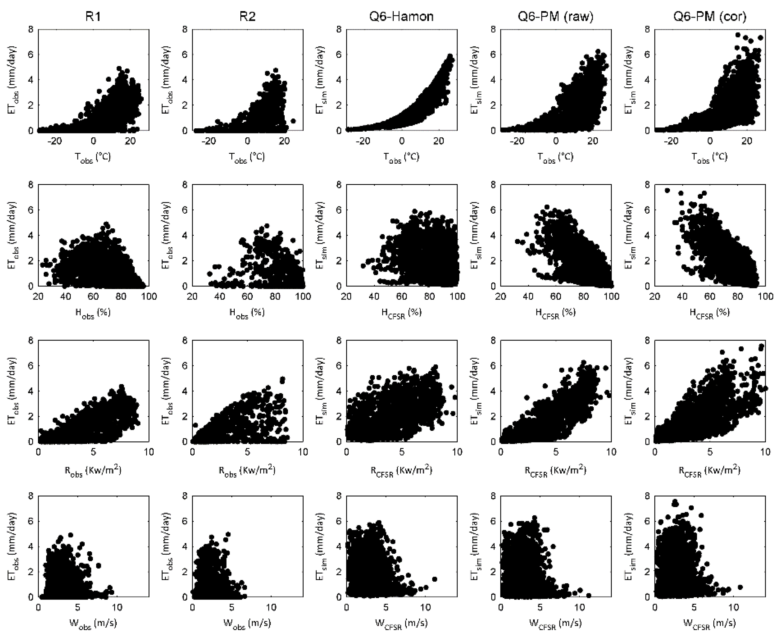
Figure 5 illustrates the 2005–2009 relations between evapotranspiration (ET) and climate drivers: air temperature, relative humidity, solar radiation, and wind speed. Relations between observed variables are also presented for sites R1 (2005–2009) and R2 (2016–2018) (Figure 1). Observed ET is inferred from latent heat flux calculated from eddy correlation measurements. Daily ET observations are generally less than 1 mm below freezing and peaks near 5 mm in summer. Above freezing, the observed ET is not strongly correlated to temperature, a notable proportion of small daily values coincide with high temperatures. The relation between observed ET and humidity decreases as humidity approaches saturation. No specific pattern emerges as humidity falls below about 75%, for which peak ET values are detected. Relation between observed ET and solar radiation reveals proportionality. ET is generally lower than 1 mm/day when radiation is below 2 kW/day, and reaches peak values above 7 kW/day. The relations between observed ET and wind speed do not present any specific pattern.
Figure 5 also presents relations between simulated ET and climate drivers. Here, ET is simulated by WaSim-ETH at site Q6 from 2005 to 2009 using Hamon and Penman-Montheith ET0 formulations. CFSR climate drivers (raw and corrected) are used, except for temperature (in situ-observation). The Hamon formulation shows a clear exponential pattern between simulated ET and temperature. It is smaller than 1 mm/day below freezing point and reaches 6 mm/day at 25 °C. Above freezing, Hamon formulation does not reproduce low ET accurately. Moreover, it does not show any clear pattern in relation with humidity, radiation, or wind speed. Relative to observations, a notable amount of overestimated ET values are found in high humidity and low radiation situations.
PM formulation forced with raw and corrected HRW fields lead to relationships in Figure 5 that are more comparable to observations than for the Hamon formulation. Low ET values above freezing are much better represented and relations between simulated ET presents proportional patterns when in relation with humidity and radiation. Correcting HRW fields moderately modifies but does not alter the broad patterns describes previously. With temperature above freezing, simulated peak ET values are emphasised while low values are overestimated. The relation between ET and humidity is shifted left while the relation with solar radiation presents a subset of values above 7 kW/day.
4. Discussion
4.1. Forcing PM Formulation with Simulated HRW Fields Provides an Appropriate Hydrologic Response
The Penman-Montheith ET0 formulation has been forced with HRW fields taken from CFSR, MERRA-2, ERA-Interim, and JRA-55 reanalyses. Hydrologic responses simulated by the WaSim-ETH model has been analyzed over six natural nivo-pluvial catchments of the St-Lawrence Valley, Canada. Results presented in Figure 3 and Figure 4 describe site-specific and reanalysis-specific hydrologic responses that are comparable to the empirical temperature-based Hamon ET0 formulation. During the nival period (December to May), 85% of the simulated hydrologic responses (41 out of 48, combined raw and corrected HRW) presented validation KGE above 0.70, generally depicting a sound representation of the spring flood in terms of synchronism, amplitude, and volume. Performance decreases during the pluvial season (June to November), 65% of the simulated hydrologic responses presenting KGE above 0.60. During that period, flow representation is affected by a systematic underestimation of the flow variance and a positive bias (Figure 4). These shortcomings are related to errors in the modeling setup, calibration failures identifying optimal parametric solutions, or misrepresentation in observations. The use of interpolated precipitation, which is known to smooth the amplitude of convective events common in summer and autumn, could explain part of the underestimation of the flow variance. The quality and resolution of the information describing soil textures could also affect seasonal water budgets and up to a certain extent the flow variance. Calibrating stomatal resistance could have potentially improved flow representation during the pluvial period.
The performance of reanalyses simulating HRW fields has been evaluated with available meteorological observations in Section 3.2. Reanalyses are generally better simulating solar radiation than humidity and wind speed. Simulated wind speed tends to present a strong systematic bias, potentially explained by the scaling mismatch between in-situ observations and the representation of the wind processes simulated at the grid-base resolution of a given reanalysis. Considering the absence of a pattern with observed evapotranspiration (Figure 5), the correction of wind may have been neglected in the scope of that study. Moreover, analysis of the meteorological performance did not identify the most successful reanalysis simulating HRW fields. Performance values are comparable for radiation while humidity and wind are marginally more accurately simulated by JRA-55 and MERRA-2. No evidence was found relating meteorological performance to the quality of the resulting hydrologic response. This can be explained by the parametric compensation allowing the search of an optimal solution indirectly correcting structural errors within the modeling setup. Taking this into account, validation of the resulting hydrologic response would be highly recommendable while using HRW fields simulated by reanalyses. These findings corroborate recent literature exploring the capacity of reanalyses to surrogate observations in providing an appropriate hydrological response [7,8,9,10,11,12,13]. They cannot highlight, as for precipitation [8,14], any strong relation between biases of raw simulated HRW fields and the quality of the resulting hydrological response.
4.2. Correcting HRW Fields Moderately Improves the Simulated Hydrologic Response
The proposed calibration-based correction has been applied to raw HRW fields in order to improve the hydrologic response. Seasonal correction factors where calibrated concomitantly to the free parameters of the hydrologic model. The correction is fairly simple to operate and does not requisite HRW observations. It relies however on the assumption that the hydrologic processes are accurate proxies of the driving climate and does not ensure the physical consistency of the corrected climate variables. In line with the work conducted by Praskievicz and Bartlein on precipitation [12], the correction provided a significant improvement of the hydrologic bias over the pluvial period (Figure 4), indicating a sensitivity of the hydrologic response to biases imprinted within HRW fields. The reduction of bias did not translate however into a significant improvement of the performance in terms of the Kling-Gupta Efficiency metric. Correction of HRW fields did not affect the simulated hydrologic responses during the nival period, except for one outlying case where correlation was highly degraded (also observed with the Hamon ET0 formulation). An in-depth analysis of the calibration intermediary results (not shown here for conciseness) revealed a calibration failure, identifying an optimal parametric solution.
4.3. PM Formulation Improves the Representation of Evapotranspiration
Within the scope of the study and according to the Wilcoxson test, the PM formulation does not provide a better hydrologic response relative to the Hamon formulation (Section 4.1), supporting findings from Sperna Weiland et al. [22]. Moreover, both formulations overestimate peak daily ET values (Figure 5), which suggests that the hydrologic model exploits the ET process to operate compensation in the representation of the annual water budget. However, the PM formulation provides a much better representation of low ET fluctuations associated to high temperatures. The latter, still imperfectly, constrains ET compelled by high humidity or low radiation driving conditions. On the other hand, the Hamon formulation suggests a sharp exponential relation between simulated ET and air temperature. It is unable to represent low ET fluctuations related to high air temperature, nor to constrain ET under high humidity or low radiation conditions. These results support the concerns raised in recent literature about the capacity of an empirical formulation such as Hamon in providing coherent projections of evapotranspiration in the scope of a non-stationary change of temperature [4,5]. The latter would potentially translate a projected steady increase of temperature into an exponential increase of ET. For these reasons, and considering potential changes in radiation and humidity, it seems recommendable to construct regional streamflow projections using physically-based ET0 formulation such as Penman-Montheith. Even if the added-value is moderate in terms of hydrologic response, it would provide a more coherent representation of daily evapotranspiration fluctuations forced by increasing air temperatures.
4.4. Limitations
To further support the recommendations previously discussed, a larger set of ET0 formulations should be analyzed. The hydrologic response is known sensible to the selection of a given ET0 formulation [1,2]. The biases of reanalyses could also be evaluated for other regions with comparable climate but more accessible data. The PM formulation is here tested in humid climate conditions, while its capacity to simulate ET can differ in more arid conditions [42]. More sophisticated HRW correction could also have been explored taking into account more resolute annual sub-scaling, quantile sorting, or multivariate dependency between corrected climate variables. Multi-seed optimization and an increase of the optimization budget could have prevented performance degradation related to correction of HRW fields. Finally, evaluating the impact of ET0 formulations within a complete climate change impact analysis was outside the scope of this study.
5. Conclusions
The manuscript demonstrated the capacity of the Penman-Montheith (PM) evapotranspiration formulation to provide a coherent hydrologic response when forced with HRW fields simulated by reanalyses. The resulting hydrologic performance remains however comparable to an empirical temperature-based evapotranspiration formulation and appears sensible to HRW biases. The manuscript also presented a calibration-based correction of simulated HRW fields free from observations. The latter improves significantly the hydrologic bias over the pluvial period (June to November) but not the overall performance according to the Kling-Gupta Efficiency (KGE) metric. Correction of HRW fields should be operated with caution since it can occasionally degrade the simulated hydrologic response. The PM formulation finally depicted much more consistent relations between evapotranspiration and climate drivers as compared to an empirical temperature-based evapotranspiration formulation. The manuscript proposes a pragmatic solution for computing evapotranspiration with physically-based formulations where HRW observations are insufficient. It also clarifies to which extent and under which conditions correcting HRW fields offers an improvement of the resulting hydrologic response. To our knowledge, few studies combine HRW fields simulated by reanalyses and observed rainfall and temperature values to force hydrologic models. This approach prevents the resulting hydrologic response to be affected by strong biases inherent to precipitation simulated by reanalyses. In the scope of most climate change studies, air temperature is expected to increase steadily according to non-stationary patterns. The main interest of the proposed approach is to compute evapotranspiration by relying on a more coherent representation of physical processes, increasing the confidence in simulated projections of the hydrologic regime.
Author Contributions
Conceptualization, S.R. and F.A.; methodology, S.R. and F.A.; software, S.R.; validation, F.A.; formal analysis, S.R.; investigation, S.R.; resources, F.A.; data curation, S.R.; writing—original draft preparation, S.R.; writing—review and editing, F.A.; visualization, S.R.; supervision, F.A.; project administration, F.A.; funding acquisition, S.R. and F.A.
Funding
This research was funded by Mitacs Accelerate program for scholarship to S.R.
Acknowledgments
The authors wish to acknowledge the contributions of Ouranos and Québec Ministry of Forests, Wildlife and Parks. This work used data from one Fluxnet-Canada site in Quebec. Fluxnet-Canada was funded by NSERC, CFCAS, Biocap-Canada, and Natural Resources Canada. Authors also wish to acknowledge Quebec Ministry of Environment and Fight Against Climate Change (MELCC) for interpolated meteorological data (precipitation and temperature), hydrometric data, digital representation of the river network and integrated description of land uses. Humidity and wind data were provided by Environment and Climate Canada. The authors thank Blaise Gauvin St-Denis and Simon Lachance-Cloutier for their support.
Conflicts of Interest
The authors declare no conflict of interest.
References
- Oudin, L.; Hervieu, F.; Michel, C.; Perrin, C.; Andréassian, V.; Anctil, F.; Loumagne, C. Which potential evapotranspiration input for a lumped rainfall-runoff model? Part 2—Towards a simple and efficient potential evapotranspiration model for rainfall-runoff modelling. J. Hydrol. 2005, 303, 290–306. [Google Scholar] [CrossRef]
- Seiller, G.; Anctil, F. How do potential evapotranspiration formulas influence hydrological projections? Hydrolog. Sci. J. 2016, 61, 2249–2266. [Google Scholar] [CrossRef] [Green Version]
- Kay, A.L.; Bell, V.A.; Blyth, E.M.; Crooks, S.M.; Davies, H.N.; Reynard, N.S. A hydrological perspective on evapotranspiration: historical trends and future projections in Britains. J. Water Clim. Chang. 2013, 4, 193–208. [Google Scholar] [CrossRef]
- Sherwood, S.; Fu, Q. A drier future? Science 2014, 343, 737–739. [Google Scholar] [CrossRef] [PubMed]
- Lofgren, B.M.; Gronewold, A.D.; Acciaioli, A.; Cherry, J.; Steiner, A.; Watkins, D. Methodological approaches to projecting the hydrologic impacts of climate change. Earth Interact. 2013, 17, 2–19. [Google Scholar] [CrossRef]
- Oudin, L.; Michel, C.; Anctil, F. Which potential evapotranspiration input for a lumped rainfall-runoff model? Part 1—Can rainfall-runoff models effectively handle detailed potential evapotranspiration inputs? J. Hydrol. 2005, 303, 275–289. [Google Scholar] [CrossRef]
- Auerbach, D.A.; Easton, Z.M.; Walter, M.T.; Flecker, A.S.; Fuka, D.R. Evaluating weather observations and the climate forecast system reanalysis as inputs for hydrologic modelling in the tropics. Hydrol. Process. 2016, 30, 3466–3477. [Google Scholar] [CrossRef]
- Essou, G.R.C.; Sabarly, F.; Lucas-Picher, P.; Brissette, F.; Poulin, A. Can precipitation and temperature from meteorological reanalyses be used for hydrological modeling? J. Hydrometeorol. 2016, 17, 1929–1950. [Google Scholar] [CrossRef]
- Fuka, D.R.; Walter, M.T.; MacAlister, C.; Degaetano, A.T.; Steenhuis, T.S.; Easton, Z.M. Using the climate forecast system reanalysis as weather input data for watershed Models. Hydrol. Process. 2014, 28, 5613–5623. [Google Scholar] [CrossRef]
- Hwang, S.; Graham, W.D.; Geurink, J.S.; Adams, A. Hydrologic implications of errors in bias-corrected regional reanalysis data for west central Florida. J. Hydrol. 2014, 510, 513–529. [Google Scholar] [CrossRef]
- Lauri, H.; Räsänen, T.A.; Kummu, M. Using reanalysis and remotely sensed temperature and precipitation data for hydrological modeling in monsoon climate: Mekong river case study. J. Hydrometeorol. 2014, 15, 1532–1545. [Google Scholar] [CrossRef]
- Praskievicz, S.; Bartlein, P. Hydrologic Modeling Using Elevationally Adjusted NARR and NARCCAP regional climate-model simulations: Tucannon River, Washington. J. Hydrol. 2014, 517, 803–814. [Google Scholar] [CrossRef]
- Seyyedi, H.; Anagnostou, E.N.; Beighley, E.; McCollum, J. Hydrologic evaluation of satellite and reanalysis precipitation datasets over a mid-latitude basin. Atmos. Res. 2015, 164–165, 37–48. [Google Scholar] [CrossRef]
- Xu, H.; Xu, C.Y.; Chen, S.; Chen, H. Similarity and difference of global reanalysis datasets (WFD and APHRODITE) in driving lumped and distributed hydrological models in a humid region of China. J. Hydrol. 2016, 542, 343–356. [Google Scholar] [CrossRef]
- Boulard, D.; Castel, T.; Camberlin, P.; Sergent, A.S.; Bréda, N.; Badeau, V.; Rossi, A.; Pohl, B. Capability of a regional climate model to simulate climate variables requested for water balance computation: A case study over northeastern France. Clim. Dyn. 2016, 46, 2689–2716. [Google Scholar] [CrossRef]
- Canon, D.J.; Brayshaw, D.J.; Methven, J.; Coker, P.J.; Lenaghan, D. Using reanalysis data to quantify extreme wind power generation statistics: A 33 year case study in Great Britain. Ren. Energy 2015, 75, 767–778. [Google Scholar] [CrossRef] [Green Version]
- Stopa, J.E.; Cheung, K.F. Intercomparison of wind and wave data from the ECMWF reanalysis interim and the NCEP climate forecast system reanalysis. Ocean Model. 2014, 75, 65–83. [Google Scholar] [CrossRef]
- Mao, Y.; Wang, K. Comparison of evapotranspiration estimates based on the surface water balance, modified penman-monteith model, and reanalysis data sets for continental China. J. Geophys. Res. Atmos. 2017, 122, 3228–3244. [Google Scholar] [CrossRef]
- Martins, D.S.; Paredes, P.; Raziei, T.; Pires, C.; Cadima, J.; Pereira, L.S. Assessing reference evapotranspiration estimation from reanalysis weather products. An application to the Iberian Peninsula. Int. J. Climatol. 2017, 37, 2378–2397. [Google Scholar] [CrossRef]
- Huang, S.Y.; Deng, Y.; Wang, J. Revisiting the global surface energy budgets with maximum-entropy-production model of surface heat fluxes. Clim. Dyn. 2017, 49, 1531–1545. [Google Scholar] [CrossRef]
- Yao, Y.; Zhao, S.; Zhang, Y.; Jia, K.; Liu, M. Spatial and decadal variations in potential evapotranspiration of china based on reanalysis datasets during 1982–2010. Atmosphere 2014, 5, 737–754. [Google Scholar] [CrossRef]
- Sperna Weiland, F.C.; Tisseuil, C.; Dürr, H.H.; Vrac, M.; Van Beek, L.P.H. Selecting the optimal method to calculate daily global reference potential evaporation from CFSR reanalysis data for application in a hydrological model study. Hydrol. Earth Syst. Sci. 2012, 16, 983–1000. [Google Scholar] [CrossRef] [Green Version]
- Jones, P.D.; Harpham, C.; Troccoli, A.; Gschwind, B.; Ranchin, T.; Wald, L.; Goodess, C.M.; Dorling, S. Using ERA-interim reanalysis for creating datasets of energy-relevant climate variables. Earth Syst. Sci. Data 2017, 9, 471–495. [Google Scholar] [CrossRef]
- Sen Gupta, A.; Tarboton, D.G. A Tool for Downscaling weather data from large-grid reanalysis products to finer spatial scales for distributed hydrological applications. Environ. Modell. Softw. 2016, 84, 50–69. [Google Scholar] [CrossRef]
- Essou, G.R.C.; Brissette, F.; Lucas-Picher, P. Impacts of combining reanalyses and weather station data on the accuracy of discharge modelling. J. Hydrol. 2017, 545, 120–131. [Google Scholar] [CrossRef]
- Mailhot, A.; Talbot, G.; Ricard, S.; Turcotte, R.; Guinard, K. Assessing the potential impacts of dam operation on daily flow at ungauged river reaches. J. Hydrol. Regional Stud. 2018, 18, 156–167. [Google Scholar] [CrossRef]
- Saha, S.; Moorthi, S.; Wu, X.; Wang, J.; Nadiga, S.; Tripp, P.; Behringer, D.; Hou, Y.T.; Chuang, H.Y.; Iredell, M.; et al. The NCEP climate forecast system version 2. J. Clim. 2014, 27, 2185–2208. [Google Scholar] [CrossRef]
- Gelaro, R.; McCarty, W.; Suárez, M.J.; Tolding, R.; Molod, A.; Takacs, L.; Randles, C.A.; Darmenov, A.; Bosilovich, M.G.; Reichle, R.; et al. The modern-era retrospective analysis for research and applications, version 2 (MERRA-2). J. Climate 2017, 30, 5419–5454. [Google Scholar] [CrossRef]
- Dee, D.P.; Uppala, S.M.; Simmons, A.J.; Berrisford, P.; Poli, P.; Kobayashi, S.; Andrae, U.; Balmaseda, M.A.; Balsamo, G.; Bauer, P.; et al. The ERA-interim reanalysis: Configuration and performance of the data assimilation system. QJR Meteorol. Soc. 2011, 137, 553–597. [Google Scholar] [CrossRef]
- Chen, G.; Iwasaki, T.; Qin, H.; Sha, W. Evaluation of the warm-season diurnal variability over east asia in recent reanalyses JRA-55, ERA-interim, NCEP CFSR, and NASA MERRA. J. Clim. 2014, 27, 5517–5537. [Google Scholar] [CrossRef]
- Kobayashi, S.; Ota, Y.; Harada, Y.; Ebita, A.; Moriya, M.; Onoda, H.; Onogi, K.; Kamahori, H.; Kobayashi, C.; Endo, H.; et al. The JRA-55 reanalysis: General specifications and basic characteristics. J. Meteorol. Soc. Jpn. 2015, 93, 5–48. [Google Scholar] [CrossRef]
- Cornelissen, T.; Diekkrüger, B.; Giertz, S. A comparison of hydrological models for assessing the impact of land use and climate change on discharge in a tropical catchment. J. Hydrol. 2013, 498, 221–236. [Google Scholar] [CrossRef]
- Ott, I.; Duethmann, D.; Liebert, J.; Berg, P.; Feldmann, H.; Ihringer, J.; Kunstmann, H.; Merz, B.; Schaedler, G.; Wagner, S. High-resolution climate change impact analysis on medium-sized river catchments in germany: an ensemble assessment. J. Hydrometeorol. 2013, 14, 1175–1193. [Google Scholar] [CrossRef]
- Smiatek, G.; Kunstmann, H.; Werhahn, J. Implementation and performance analysis of a high resolution coupled numerical weather and river runoff prediction model system for an alpine catchment. Environ. Modell. Softw. 2012, 38, 231–243. [Google Scholar] [CrossRef]
- Allen, R.G.; Pereira, L.S.; Raes, D.; Smith, S. Crop Evapotranspiration—Guidelines for Computing Crop Water Requirements; Irrigation and Drainage Paper 56; FAO: Rome, Italy, 1998; pp. 1–15. [Google Scholar]
- Shangguan, W.; Dai, Y.; Duan, Q.; Liu, B.; Yuan, H. A global soil data set for earth system modeling. J. Adv. Model. Earth Syst. 2014, 6, 249–263. [Google Scholar] [CrossRef]
- Asadzadeh, M.; Tolson, B.A. Hybrid pareto archived dynamically dimensioned search for multi-objective combinatorial optimization: application to water distribution network design. J. Hydroinform. 2012, 14, 192–205. [Google Scholar] [CrossRef]
- Gupta, H.V.; Kling, H.; Yilmaz, K.K.; Martinez, G.F. Decomposition of the mean squared error and nse performance criteria: Implications for improving hydrological modelling. J. Hydrol. 2009, 377, 80–91. [Google Scholar] [CrossRef]
- Wilcoxon, F. Individual comparisons by ranking methods. Biometrics 1945, 1, 80–83. [Google Scholar] [CrossRef]
- Muerth, M.J.; Gauvin St-Denis, B.; Ricard, S.; Velázquez, J.A.; Schmid, J.; Minville, M.; Caya, D.; Chaumont, D.; Ludwig, R.; Turcotte, R. On the need for bias correction in regional climate scenarios to assess climate change impacts on river runoff. Hydrol. Earth Syst. Sci. 2013, 17, 1189–1204. [Google Scholar] [CrossRef] [Green Version]
- Velázquez, J.A.; Schmid, J.; Ricard, S.; Muerth, M.J.; Gauvin St-Denis, B.; Minville, M.; Caya, D.; Chaumont, D.; Ludwig, R.; Turcotte, R. An ensemble approach to assess hydrological models’ contribution to uncertainties in the analysis of climate change impact on water resources. Hydrol. Earth Syst. Sci. 2013, 17, 565–578. [Google Scholar] [CrossRef]
- Hajji, I.; Nadeau, D.F.; Music, B.; Anctil, F.; Wang, J. Application of the maximum entropy production model of evapotranspiration over partially vegetated water-limited land surfaces. J. Hydrometeorol. 2019, 19, 989–1005. [Google Scholar] [CrossRef]
Figure 1.
Location of the outlet of the six catchments (circles) and of the nearest meteorological stations (triangles and squares) from which humidity, radiation and wind speed observations are extracted.
Figure 1.
Location of the outlet of the six catchments (circles) and of the nearest meteorological stations (triangles and squares) from which humidity, radiation and wind speed observations are extracted.

Figure 2.
Calibration-based correction of HRW fields taken from reanalyses. Seasonal correction factors are calibrated concomitantly to the hydrologic model according to an objective-function, the latter minimizes deviation between observed and simulated streamflow.
Figure 2.
Calibration-based correction of HRW fields taken from reanalyses. Seasonal correction factors are calibrated concomitantly to the hydrologic model according to an objective-function, the latter minimizes deviation between observed and simulated streamflow.

Figure 3.
Observed and simulated 2008 hydrographs at sites Q1 to Q6. Hydrographs are simulated with raw HRW fields taken from CFSR, MERRA-2, ERA-Interim, and JRA-55 reanalyses.
Figure 3.
Observed and simulated 2008 hydrographs at sites Q1 to Q6. Hydrographs are simulated with raw HRW fields taken from CFSR, MERRA-2, ERA-Interim, and JRA-55 reanalyses.

Figure 4.
Hydrologic performance of the Penman-Montheith formulation forced with raw and corrected HRW fields. These latter are taken from reanalyses CFSR, MERRA-2, ERA-Interim, JRA-55 at sites Q1 to Q6 (n = 24). Performance is assessed through KGE and α, β, r components evaluated from December to May (DJFMAM) and from June to November (JJASON). KGE values are ventilated for each reanalysis and compared to the Hamon temperature-based ET0 formulation (n = 6).

Figure 5.
Relations between evapotranspiration (ET) and climate drivers: temperature (T), humidity (H), radiation (R), and wind speed (W). All variables are observed at sites R1 and R2. At site Q5, ET is simulated by WaSim-ETH with Hamon and PM formulations. T is observed and HRW are taken from CFSR reanalysis (raw and corrected).


Table 1.
Description of hydrometric stations.
| Site | Latitude (°N) | Longitude (°E) | Area (km2) | Forest Land Use (%) | Slope (%) | Corresponding Meteorological Station |
|---|---|---|---|---|---|---|
| Q1 | 47.6 | −69.7 | 512 | 77 | 5.9 | M1 |
| Q2 | 46.2 | −70.6 | 695 | 75 | 4.1 | M2 |
| Q3 | 45.8 | −72.0 | 549 | 60 | 5.8 | M3 |
| Q4 | 45.6 | −71.4 | 736 | 79 | 7.9 | M3 |
| Q5 | 45.9 | −73.5 | 633 | 59 | 6.4 | M4 |
| Q6 | 46.6 | −73.2 | 761 | 83 | 13.4 | M5 |
Table 2.
Hydrologic modeling setup.
| Hydrologic Process | Description | Climate Input Data | Free Parameters |
|---|---|---|---|
| ET0 | Penman-Monteith | Temperature Humidity Radiation Wind speed | none |
| Hamon | Temperature | fi [0.5;2] | |
| Precipitation correction | Separation liquid/solid precipitation | Temperature Precipitation | Ttr [−0.5;0.5] as [1;1.5] |
| Snow melt | T-Index degree day method | Temperature | c0 [0;5] Tm [−2;2] |
| Unsaturated zone fluxes | Surface runoff generation | None | QDsnw [0;1] |
| Interflow generation | None | dr [1;100] | |
| Discharge routing | Surface and interflow flow recession | None | ks [1;100] kh [1;150] |
Table 3.
Meteorological performance of CFSR, MERRA-2, ERA-Interim and JRA-55 simulating humidity, radiation and wind speed observations. Performance is expressed through the Kling-Gupta efficiency metric (KGE) and its related component (α, β and r) evaluated from June to November.
Table 3.
Meteorological performance of CFSR, MERRA-2, ERA-Interim and JRA-55 simulating humidity, radiation and wind speed observations. Performance is expressed through the Kling-Gupta efficiency metric (KGE) and its related component (α, β and r) evaluated from June to November.
| CFSR | MERRA-2 | ERA-Interim | JRA-55 | M | R | |
|---|---|---|---|---|---|---|
| Humidity | ||||||
| KGE | 0.66 | 0.64 | 0.62 | 0.70 | 0.65 | 0.07 |
| α | 1.19 | 0.82 | 1.25 | 1.04 | 1.07 | 0.43 |
| β | 1.01 | 1.05 | 0.94 | 0.98 | 0.99 | 0.11 |
| r | 0.72 | 0.70 | 0.73 | 0.71 | 0.71 | 0.02 |
| Radiation | ||||||
| KGE | 0.84 | 0.90 | 0.89 | 0.88 | 0.88 | 0.06 |
| α | 1.03 | 0.98 | 0.96 | 0.96 | 0.98 | 0.07 |
| β | 0.92 | 1.07 | 1.07 | 1.09 | 1.04 | 0.17 |
| r | 0.87 | 0.93 | 0.93 | 0.93 | 0.91 | 0.06 |
| Wind speed | ||||||
| KGE | 0.40 | 0.63 | 0.43 | 0.44 | 0.48 | 0.23 |
| α | 1.47 | 0.74 | 1.35 | 0.62 | 1.05 | 0.84 |
| β | 1.26 | 0.87 | 1.36 | 0.67 | 1.04 | 0.69 |
| r | 0.77 | 0.82 | 0.77 | 0.79 | 0.79 | 0.05 |
Table 4.
Optimized values of WaSim-ETH free parameters.
| Parameters | Hamon (n = 6) | PM Raw (n = 24) | PM Cor (n = 24) | |||||
|---|---|---|---|---|---|---|---|---|
| Equation | Mean | [Min;Max] | Mean | [Min;Max] | Mean | [Min;Max] | ||
| fi,DJFMAM | Correction of Hamon ET0 | (3) | 0.96 | [0.50;1.42] | - | - | - | - |
| fi,JJASON | 1.26 | [1.14;1.40] | - | - | - | - | ||
| Ttr | Temperature snow/rain transition | (4) | 0.42 | [0.23;0.5] | 0.0063 | [−0.5;0.5] | 0.22 | [−0.44;0.5] |
| as | Correction of solid precipitation | (4) | 1.28 | [1.18;1.5] | 1.17 | [1;1.49] | 1.26 | [1;1.49] |
| c0 | Melt factor | (5) | 2.61 | [1.41;3.99] | 2.42 | [0.6;5] | 2.53 | [1.11;5] |
| Tm | Temperature limit for snow melt | (5) | −1.56 | [−2;0.18] | −0.47 | [−2;2] | −0.95 | [−2;1.71] |
| QDsnw | Fraction of surface runoff on snow melt | (6) | 0.51 | [0;1] | 0.67 | [0;1] | 0.40 | [0;1] |
| dr | Drainage density | (7) | 81.50 | [40.29;100] | 33.55 | [1;100] | 73.12 | [1;100] |
| ks | Surface runoff recession constant | (8) | 78.94 | [51.33;100] | 73.49 | [28.80;100] | 66.24 | [30.36;100] |
| kh | Inteflow recession constant | (9) | 45.87 | [16.65;139.82] | 50.68 | [11.81;150] | 50.08 | [10.36;150] |
© 2019 by the authors. Licensee MDPI, Basel, Switzerland. This article is an open access article distributed under the terms and conditions of the Creative Commons Attribution (CC BY) license (http://creativecommons.org/licenses/by/4.0/).
Share and Cite
MDPI and ACS Style
Ricard, S.; Anctil, F. Forcing the Penman-Montheith Formulation with Humidity, Radiation, and Wind Speed Taken from Reanalyses, for Hydrologic Modeling. Water 2019, 11, 1214. https://doi.org/10.3390/w11061214
AMA Style
Ricard S, Anctil F. Forcing the Penman-Montheith Formulation with Humidity, Radiation, and Wind Speed Taken from Reanalyses, for Hydrologic Modeling. Water. 2019; 11(6):1214. https://doi.org/10.3390/w11061214
Chicago/Turabian StyleRicard, Simon, and François Anctil. 2019. "Forcing the Penman-Montheith Formulation with Humidity, Radiation, and Wind Speed Taken from Reanalyses, for Hydrologic Modeling" Water 11, no. 6: 1214. https://doi.org/10.3390/w11061214
Note that from the first issue of 2016, this journal uses article numbers instead of page numbers. See further details here.