Article

Energy Reduction and Uniformity of Low-Pressure Online Drip Irrigation Emitters in Field Tests

1
Department of Mechanical Engineering, Massachusetts Institute of Technology, Cambridge, MA 02139, USA
2
International Center for Agricultural Research in the Dry Areas, Rabat 10100, Morocco
3
Civil Engineering Department, Jordan University of Science and Technology, Irbid 22110, Jordan
4
Methods for Irrigation and Agriculture, Amman 11194, Jordan
5
Institut National de la Recherche Agronomique, Rabat 10090, Morocco
6
National Agricultural Research Center, Amman 19381, Jordan
*
Author to whom correspondence should be addressed.
Water 2019, 11(6), 1195; https://doi.org/10.3390/w11061195
Submission received: 21 May 2019 / Revised: 4 June 2019 / Accepted: 5 June 2019 / Published: 7 June 2019
(This article belongs to the Special Issue Precision Agriculture and Irrigation)

Abstract

:
A promising way of addressing the issue of growing water scarcity is through wider use of drip irrigation, which delivers water and fertilizer to crops in a slow, targeted manner, and has been shown to increase yields and water use efficiency. Yet, drip irrigation system adoption is low, primarily due to the high capital cost of the pressurized piping network and the pump, and operating energy cost. Lowering the water pressure needed for drip emitters to deliver water can reduce both capital and operating costs of drip systems. Here we present the results from field trials of new pressure-compensating online drip emitters that operate with a minimum compensating inlet pressure of 15 kPa (0.15 bar), in comparison to typical commercial emitters with minimum pressures of 50–100 kPa (0.5–1.0 bar). The field trials were carried out on nine farms in Morocco and Jordan over the course of one irrigation season with freshwater and treated wastewater. Low-pressure emitters are shown to reduce hydraulic energy per unit volume of water delivered by 43% on average compared to commercial emitters, without significantly sacrificing water emission uniformity (low-pressure emitters show uniformities of 81–91%, compared to 87–96% for commercial emitters). This energy reduction could lead to savings of 22–31% in the capital cost of a pump and emitters and the energy cost for a typical drip irrigation system. Thus, the low-pressure online emitters can be used as substitutes to commercial emitters that require higher water pressures, leading to reduced environmental impact and lower system costs.

Graphical Abstract

1. Introduction

Rising global water scarcity is limiting the growth of agricultural productivity, especially in arid regions [1]. Drip irrigation is an underutilized method of irrigation that can raise crop productivity and save water for the farmer, compared to flood irrigation, the most common method used in the region [2]. A drip irrigation system delivers water in a slow, targeted manner through a network of pipes with drip emitters laid out along rows of crops, reducing water lost to evaporation and deep percolation. It allows greater control over the rate and amount of water and fertilizer application and enables water-saving and yield-increasing strategies such as deficit or supplemental irrigation. When best practices are applied, drip irrigation has been shown to reduce water use by 9–70% and improve crop yields by 8–50% compared to flood irrigation [2,3,4,5].
In spite of its benefits, drip irrigation is currently used on only 6% of irrigated land, compared to sprinkler (17%) and flood irrigation (77%) [6]. Several drawbacks limit its wide adoption. A major drawback is capital cost: Unlike flood irrigation, which only needs a low-pressure pump (or none at all, if water is delivered from a higher elevation), drip irrigation requires a pressurized pipe network that reaches every plant, plus drip emitters, filters to prevent clogging of the emitters, and a higher-pressure pump to counteract the head losses throughout the entire system. In locations where grid electricity is unreliable or unavailable, a diesel generator or an off-grid solar power system is needed to operate the pump, further increasing the capital cost. For solar-powered drip irrigation systems, the pump and photovoltaic array can account for up to 80% of the total cost [7]. For grid-connected or diesel-powered drip systems, the recurring electricity or diesel cost for pumping can be a significant expense to the farmer.
The largest contributors to pressure losses in a drip irrigation system are usually the drip emitters themselves, especially in the case of pressure-compensating (PC) emitters [7]. PC emitters maintain a nearly constant flow rate regardless of variation in water pressure, as long as that pressure is above the Minimum Compensating Inlet Pressure (MCIP) (Figure 1). PC operation is beneficial to crops, as it results in a uniform distribution of water to all parts of the field, in contrast to non-PC emitters, which decrease flow at lower water pressures in areas farther from the pump. Most commercially-available PC emitters have a minimum operating pressure of 50–100 kPa (0.5–1.0 bar). Once additional pressure losses in piping, filters, and fertigation systems are accounted for, the required pump outlet pressures for a surface water source are on the order of 150–200 kPa (1.5–2 bar) or greater, depending on field size. Significantly reducing the MCIP of PC emitters may, therefore, reduce the pump capacity and its power requirement, leading to lower capital costs for the pump, as well as lower capital costs for the power supply of off-grid systems or a reduced recurring electricity cost for grid-connected systems.
With the goal of reducing the capital and operating costs of drip irrigation systems, Shamshery et al. [8] developed an analytical model based on a commercial online PC emitter produced by Jain Irrigation Ltd., then employed a genetic algorithm to optimize its geometry to reduce the MCIP while maintaining PC behavior [7]. The optimization for an emitter with a flow rate of 8.2 liters per hour (L/h) produced a design with an MCIP of 15 ± 5 kPa (0.15 ± 0.05 bar) and a reduction of 83% from the MCIP of 90 kPa (0.90 bar) for Jain’s commercial PC emitter. After the design was validated by laboratory testing, a batch of low-pressure emitters was manufactured by Jain Irrigation Ltd. using their standard injection molding process.
This paper describes field trials designed to assess the performance of these new low-pressure online PC emitters on farms in arid regions in the Middle East and North Africa, the most water-stressed region in the world [9]. Experiments were conducted in Jordan and Morocco—two countries in the region that rely heavily on agriculture and are dealing with increasing water stresses due to reduction in precipitation, aquifer depletion, and population growth [9,10]. In Morocco, approximately 10% of the irrigated area is under drip irrigation [11]. In response to growing water shortages, the Moroccan government launched the Green Morocco Plan (Plan Maroc Vert) in 2008 to modernize national agriculture, increase its productivity, and reduce water waste [12,13]. This will be done by disseminating drip irrigation to approximately half of the irrigated area by the year 2022 through subsidies offered to individual farmers and farmer collectives [14]. In Jordan, an estimated 81% of irrigated land already uses drip or other localized irrigation [15]. Due to the scarcity of renewable freshwater in Jordan (groundwater is being used at twice the rate at which it is recharged), 26% of the water used for irrigation is treated wastewater, and wastewater treatment capacity continues to increase [16,17]. Thus, it is important to assess the performance of drip emitters with treated wastewater in addition to canal and groundwater sources.
The goals of the field trials in Jordan and Morocco were to compare the performance of low-pressure online PC emitters (henceforth referred to as low-pressure emitters) to that of locally-available commercially-sold online PC emitters (referred to as conventional emitters). Specifically, they aimed to (1) quantify the energy reduction due to the use of low-pressure emitters when compared to locally-available conventional emitters; (2) measure the water distribution uniformity of low-pressure emitters over the course of an irrigation season, and compare it to the uniformity of conventional emitters, when both are operated at or above their MCIP; and (3) compare the uniformity of low-pressure and conventional emitters when operated at conventional pressures using treated wastewater (in Jordan only). We describe the results of the field trials and their implications in terms of cost savings for farmers who may choose to use the low-pressure emitters.

2. Materials and Methods

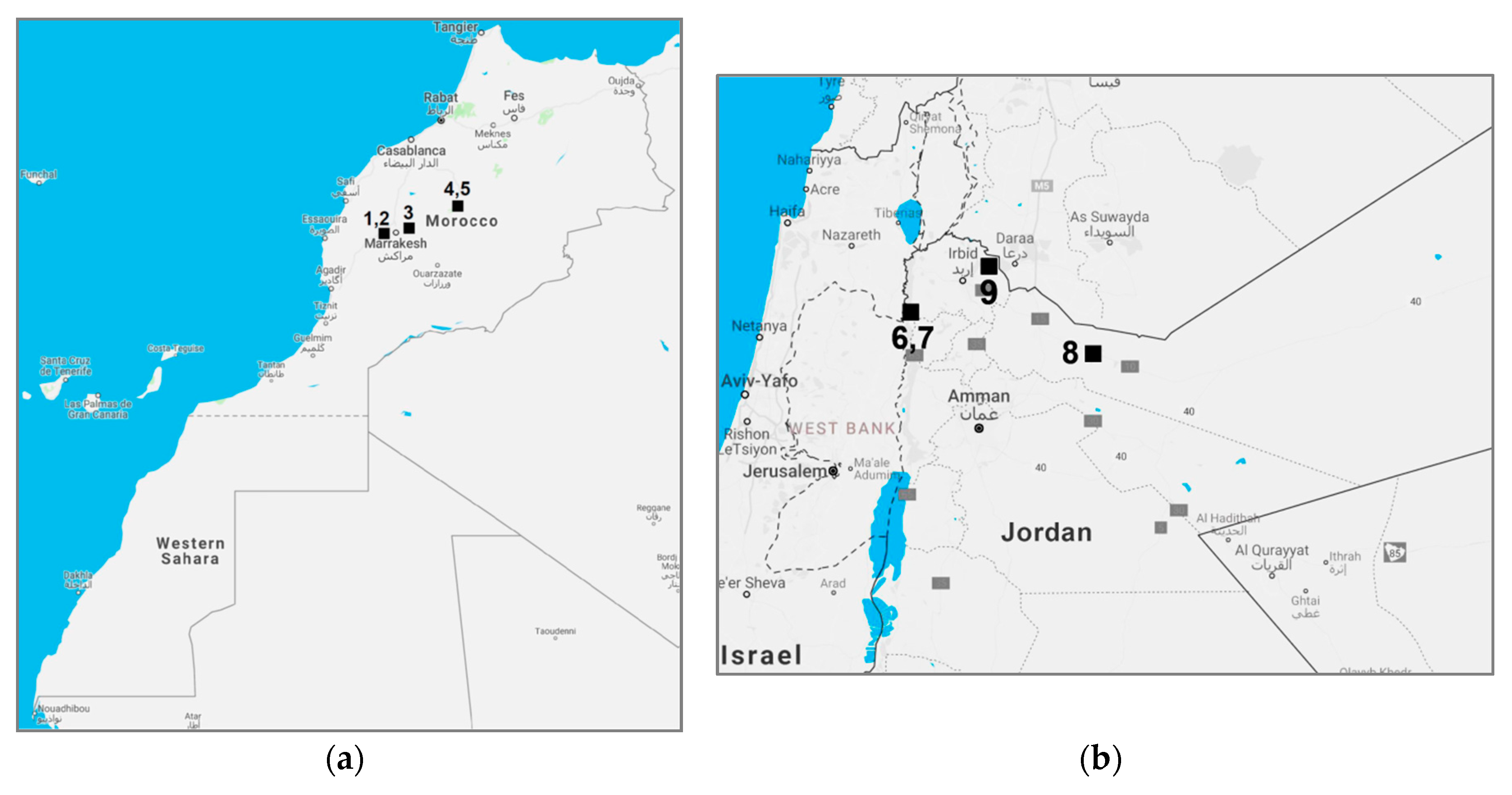
2.1. Experimental Sites

Experiments were conducted at three locations in Morocco and three locations in Jordan (Figure 2), with one or two experimental sites at each location. The experimental drip irrigation systems were managed by researchers at the International Center for Agriculture in Dry Areas (ICARDA) and the Institut National de la Recherche Agronomique (INRA) in Morocco, and by Methods for Irrigation and Agriculture (MIRRA) and the National Agricultural Research Center (NARC) in Jordan. In each country, the locations included one private farm and two or more research stations belonging to the government agricultural research institutes—INRA in Morocco and NARC in Jordan. A list of all experimental sites is provided in Table 1, with typical weather statistics and irrigation water properties. The chosen locations featured a range of water sources (groundwater wells, canal water, treated wastewater) with varying quality and clogging potential, selected to evaluate the performance of low-pressure emitters under different conditions. Water quality at each site was measured one or more times throughout the irrigation season (see Section 2.5.3).
Two methodologies were used on the sites: One for sites using freshwater, another for the site using treated wastewater. The methodologies are described in more detail in Section 2.2 and Section 2.3, respectively. Instrumentation and data loggers were installed at all sites in May 2017. Sensor and manual data measurements were conducted from June 1 until the last irrigation events in December 2017. Several gaps in sensor data during that time period are a result of sensor or data logger malfunctions, such as corrosion of the spinning paddlewheel of the flow sensors, or temporary loss of power.

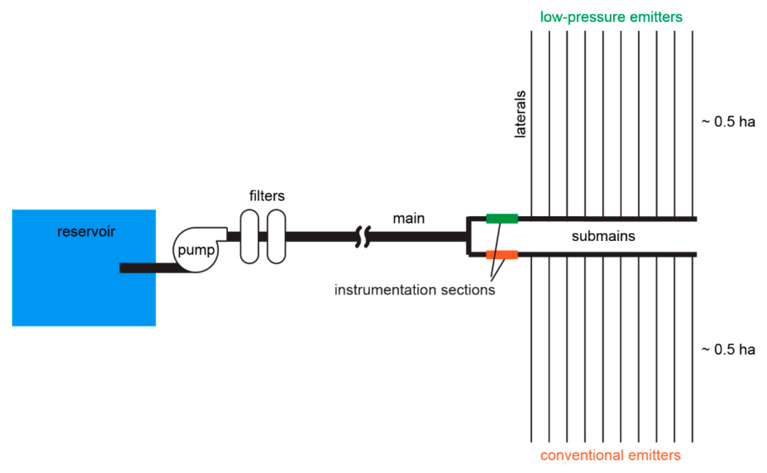
2.2. Experimental Setup for Measurement of Emitter Performance with Freshwater

At the sites using freshwater, irrigation was conducted on tree crops (citrus, pomegranates, or olives) of different ages. The crops were irrigated regularly between April and December 2017, with the schedule set by the farm managers according to crop water requirements calculated using the Penman-Monteith method with historical local weather averages. Throughout the season, irrigation durations were adjusted from pre-calculated ones when needed, based on precipitation and any departures from historical weather patterns.
Each freshwater site with tree crops was divided into two plots of approximately equal area (Table 2). One plot was outfitted with low-pressure online PC emitters, and the other plot was outfitted with conventional online PC emitters widely used in that region. The conventional emitters were used as the control scenario reflecting typical local practices. The two models of conventional emitters used in experiments are labeled as emitters A in Morocco and B in Jordan. Online emitters were used at all sites to accommodate the wide spacing between the trees in each row, which ranged between 3 and 8 m. All emitters were manually installed in brand new laterals, with two or more emitters at each tree, depending on the tree’s age and water requirement. While the areas of the two plots at each site were kept consistent, the number of trees was not always identical between plots because the experiments were constrained by existing crop locations. The differences in tree numbers between plots of the same area can be attributed to missing trees that had been removed prior to the experiment, or uneven numbers of laterals available for the experiment. Due to the differences in numbers of trees and emitters between two plots at one site, the water volume delivered to each plot was not expected to be identical; therefore, the hydraulic energy measurements were normalized by the volume of water delivered to each plot (see Section 2.6).
Water was delivered to both plots by the same pump, via a main pipe that branched into multiple submain pipes (Appendix B Figure A1). Each plot was served by its own submain. At the start of each submain, a valve section was installed, containing a manual valve for pressure regulation and a series of sensors. The manual valves were locally-purchased ball valves of the same diameter as the submain pipe. These valves were used due to the lack of availability of pressure-regulating valves at the high flow rates and low pressures needed for the experiments. Due to the constant-flow characteristic of PC emitters, manual valves were not expected to affect flow rates when all emitters were operating above the MCIP. The pressure in each submain was manually set to the minimum recommended operating pressure for that emitter type. The following procedures were followed to set the minimum operating pressures for plots with the two emitter types:
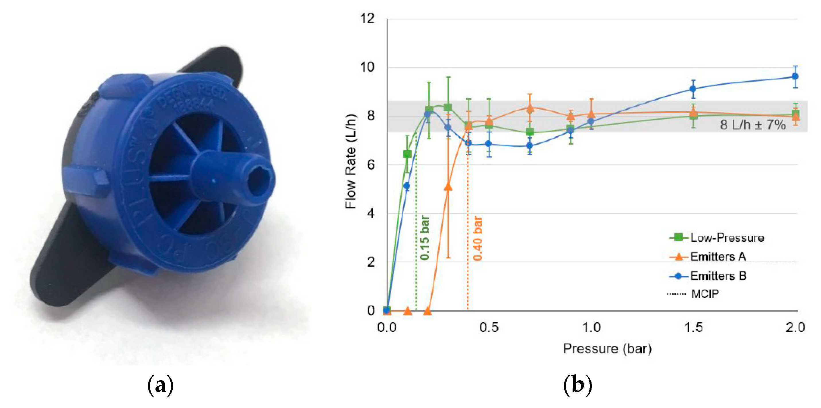
  • Conventional emitters: The submain pressure was reduced until the pressure at the end of the farthest lateral was above the minimum emitter operating pressure, as recommended by the emitter manufacturer.
  • Low-pressure emitters: The submain pressure was reduced until the average flow rate from the farthest five emitters was within ±10% of the nominal flow rate. Nominal flow rate was deemed an appropriate metric because these emitters are not sold commercially and, hence, do not have a manufacturer-recommended operating pressure.
The minimum operating pressure settings determined by this procedure, as well as the crop type and age, number of trees, and number of emitters for each plot are listed in Table 2. Actual operating pressures sometimes diverged from these minimum settings due to unpredictable variations in system operation over time, such as opening and closing of valves on non-experimental plots connected to the piping system, or staff intervention. They were reset to the minimum pressure setting before each uniformity measurement was taken. (See Section 3.1 for full details on actual operating pressures.)
Irrigation system maintenance was performed by farm staff according to their regular maintenance procedures, which included filter cleaning and system flushing. More details are provided in Appendix A.1.

2.3. Experimental Setup for Measurement of Emitter Performance with Treated Wastewater

One experimental site, Ramtha Research Station in Jordan, was situated next to the Ramtha city wastewater treatment plant, which processes domestic wastewater using the sludge-extended aeration treatment process. Treated wastewater from this plant was used to conduct an experiment on the uniformity of low-pressure and conventional emitters operated at different pressures using treated wastewater as a source. Due to the high clogging potential associated with treated wastewater, a field without crops was used for the experiment. Irrigation was conducted on a set schedule for 3 h a week regardless of weather.
A pump delivered the treated wastewater from a reservoir through a sand and disk filter, then through one main pipe to the field, where it branched into three submains (Appendix B Figure A2). A pressure-regulating valve at the start of each submain was used to set a different pressure for each: 25, 50, and 100 kPa (0.25, 0.5, and 1 bar). The submains at 50 and 100 kPa (0.5 and 1 bar) delivered water to 16 laterals each—eight with low-pressure emitters, eight with conventional emitters. The submain at 25 kPa (0.25 bar) delivered water to 16 laterals with low-pressure emitters only, because it was far below the recommended operating pressure for conventional emitters. Approximately 40 emitters were installed on each lateral. Systems were maintained according to standard practice. Full details of system maintenance are described in Appendix A.1.

2.4. Emitter Characteristics

The low-pressure emitters were designed by Shamshery and Winter [7] and manufactured by Jain Irrigation Ltd. at its injection molding plant in Jalgaon, India (Figure 3a). Conventional emitters used as controls were purchased locally from market-leading manufacturers and are labeled as emitters A in Morocco and emitters B in Jordan. Both emitter models were PC online emitters with nominal flow rates of 8.0 L/h and had the lowest MCIPs of commercially-available emitters with that flow rate. Due to limited local availability in Morocco, a mix of PC and PC-NL (non-leakage) versions of emitters A were installed. The non-leakage emitters have features that prevent water flow below 12 kPa (0.12 bar), according to the specification sheet.
A random sample of 25 new emitters from each type was tested in the laboratory for flow-pressure performance and the manufacturing coefficient of variation ( C V m ) following Standard ISO 9261:2004 [21]. This laboratory test was conducted in order to characterize the emitters according to standard industry practice. Inlet pressure to the tubes with the 25 emitters was measured with a pressure gauge (DPGW-07, Dwyer, Michigan City, IN, USA, ±3 kPa) and varied in the range 10–300 kPa (0.1–3.0 bar). At each test pressure, flow rate from all emitters was measured by allowing water to drip into empty containers for 2.00 min, then weighing the filled containers on a scale (ScoutPro, Ohaus, Parsippany, NJ, USA, ±0.01 g) and subtracting the initial empty weight of the containers.
The characteristic flow versus pressure curves for all emitters are shown in Figure 3b. Laboratory tests indicated that the low-pressure emitters had an MCIP of 15 ± 5 kPa (0.15 ± 0.05 bar) and a nominal flow rate of 8.0 L/h (MCIP is defined as the minimum pressure at which the emitter’s flow rate is within ± 7% of the nominal flow rate). The sample of emitters A, consisting of PC-NL emitters only, had an MCIP of 40 ± 5 kPa (0.40 ± 0.05 bar) with the same nominal flow rate. The minimum operating pressure recommended by the manufacturer includes a small safety factor to account for manufacturing variation and is thus slightly higher than the measured MCIP: 50 kPa (0.5 bar) for PC and 70 kPa (0.7 bar) for PC-NL emitters. The lower of these was used as the target operating pressure in the field, since the laboratory test of PC-NL emitters showed that nominal flow rates were already reached at 50 kPa (0.5 bar). The sample of emitters B revealed a lack of true pressure compensation, as the flow did not level out around 8 L/h but continued to increase with pressure. For these emitters, the lowest pressure at which the nominal flow rate was reached was 15 kPa (0.15 bar), but then the flow rate dipped below the nominal range, reaching it again at 95 ± 5 kPa (0.95 ± 0.05 bar). Thus, the MCIP of emitters B was undefined, and the minimum field operating pressure was based on the manufacturer’s specification of 100 kPa (1.0 bar).
The manufacturing coefficients of variation ( C V m ) over a range of pressures for the low-pressure emitters was also measured following ISO Standard 9261:2004 [21]. The results of C V m measurements (Figure 10) and their relation to water emission uniformity are discussed in Section 4.2.

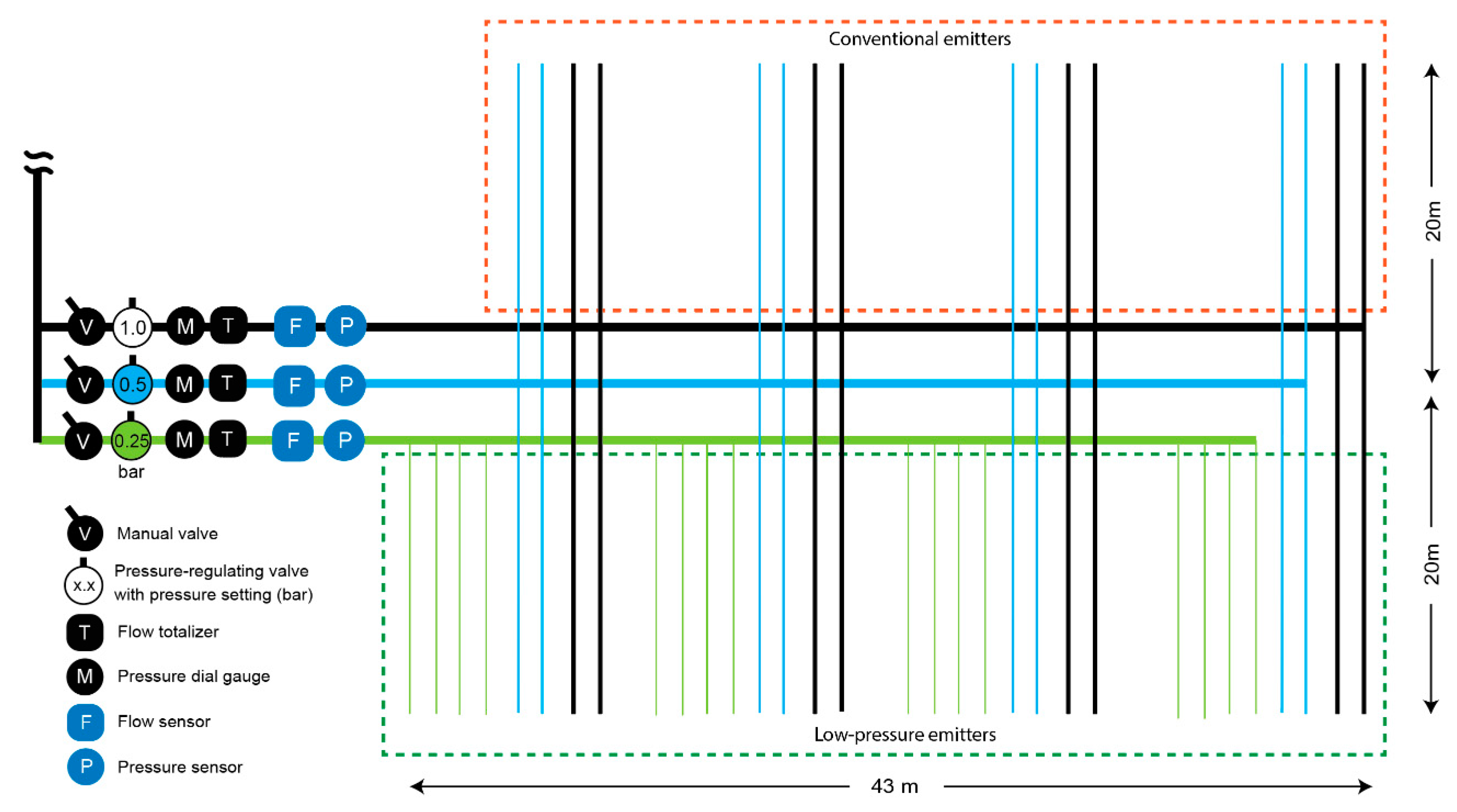
2.5. Experimental Measurements

Three types of measurements were conducted throughout the irrigation season: (1) electronic sensor measurements of water pressure and flow rate in the submain; (2) uniformity, calculated from manual measurements of flow rates from a subset of emitters; (3) analysis of water quality. One or more of these measurement types was conducted at each site (Table 2). Details of each measurement procedure are presented below.

2.5.1. Pressure and Flow Sensor Measurements

One pressure sensor (MediaSensor P51, SSI, Janesville, WI, USA, ±3 kPa) and one flow sensor (DFMT-25A, Dwyer, Michigan City, IN, USA on sites 1 and 5; PFT, Dwyer, Michigan City, IN, USA on sites 2–3, 6–9) were installed on each submain downstream of the pressure-regulating valve. All sensors were calibrated during field installation (detailed in Appendix A.2). Several flow sensors experienced corrosion over time, which inhibited the functionality of the paddlewheel mechanism; when this issue was noticed, the flow sensors were cleaned and re-calibrated by field staff.
Analog dial pressure gauges were installed side-by-side with the electronic pressure sensors, for use by research staff when setting the operating pressures on the submain. Dial pressure gauges were purchased locally and had a maximum measurement and reading error of ±10 kPa. Analog water totalizers were installed next to flow sensors and used for flow sensor calibration; all models and manufacturers are listed in Appendix A.2.
The sensors on each submain were connected to a custom Arduino-based data logger (16-bit analog-to-digital conversion) programmed to read sensor outputs every 30 s and save them to CSV files. The data logger also transmitted 10-minute averaged sensor values via a cellular network to a server in real time, so the researchers could monitor sensor readings remotely and troubleshoot promptly.

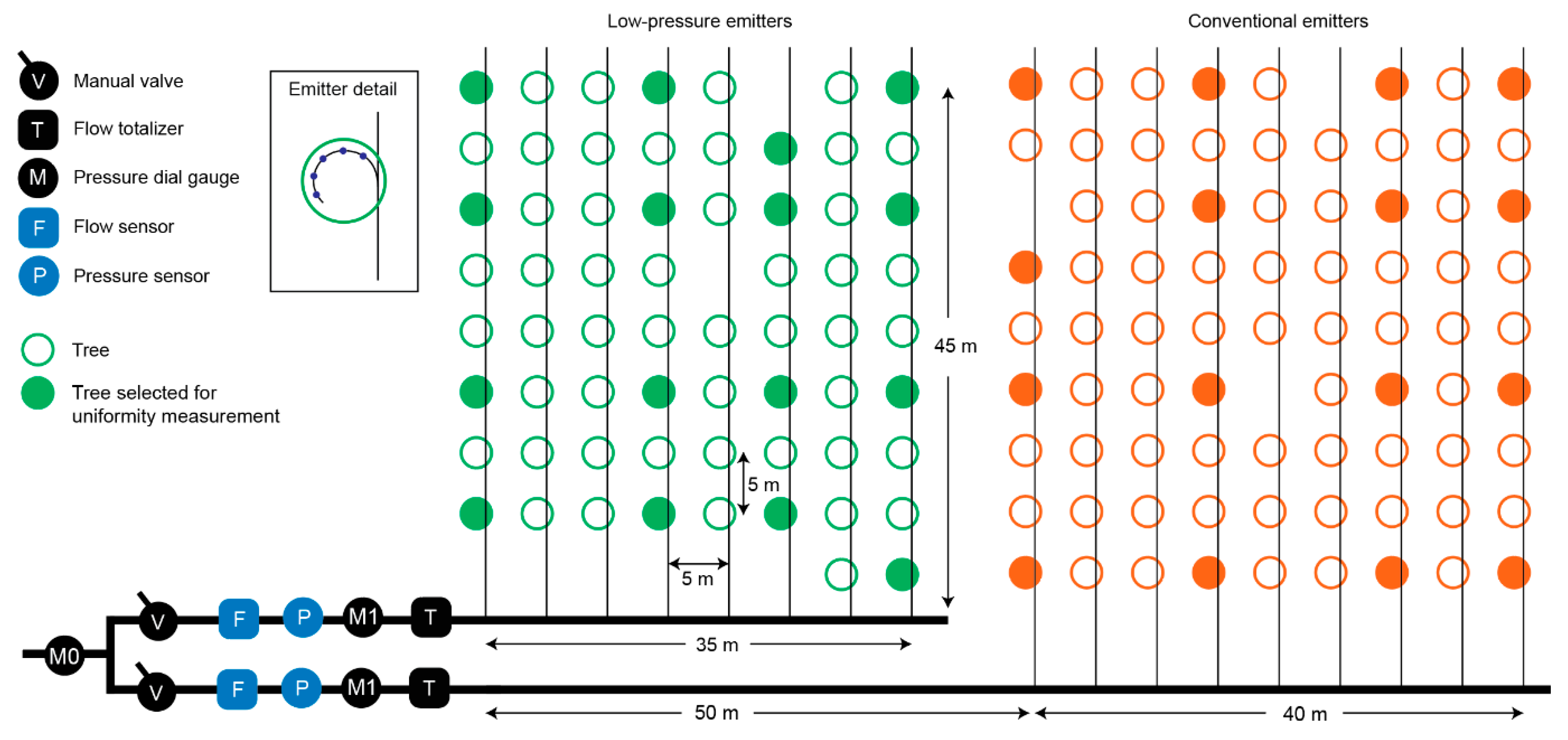
2.5.2. Uniformity Measurement

Water emission uniformity in the field was measured over the course of the irrigation season to evaluate the combined effects of manufacturing variation, hydraulic pressure variation, and clogging. Every 2–4 weeks, the researchers recorded flow rate measurements from 32 emitters at every plot. The 32 emitters were distributed throughout the plot as follows (Figure 4): (1) The plot was divided into quarters along its width and length; (2) one tree was selected within each section, for a total of 16 trees; (2) two neighboring emitters at each of the 16 trees were selected. The flow rate was measured by placing a container under each emitter, timing it for 5 min or more, and measuring the final volume of water in the container using a graduated cylinder. The flow rate was calculated by dividing the water volume by the measurement time period, with an uncertainty of ±0.08 L/h (1% of the nominal 8 L/h flow rate of all emitters).
Recorded emitter flow rates from 32 emitters on each plot were used to calculate water application uniformity using the metric of statistical uniformity (SU) according to Equation (1) [22,23]:
S U = ( 1 S q q ¯ ) × 100 % ,
where q ¯ is the mean flow rate of all emitters (L/h) and S q is the standard deviation of all measured flow rates (L/h). The sample size of 32 emitters exceeds the industry-recommended minimum sample size of 18, in order to reduce the standard error of the SU measurement [22,24]. The standard error of each measurement was calculated and is reported with the results.
In the course of the emitter flow rate measurements, when research staff encountered an emitter with a visibly reduced flow rate (an indication of clogging), its flow rate was recorded as usual. After the measurement, the staff either repaired the emitter by tapping on it to dislodge solid particles or by unscrewing the cap and cleaning the inside. Conventional emitters used in Morocco did not feature a removable cap, so they could only be fixed by tapping, by temporarily blocking the outlet to create a localized pressure increase, or by using a suction pump. At sites 3 and 4 in Morocco (Beni Mellal Research Station), clogged emitters were sometimes repaired by applying an acid solution externally into the emitter outlet orifice. If repair attempts were unsuccessful, the emitter was replaced with a new one of the same type. The cleaning and replacement procedure was followed for all emitters in the field and is indicative of typical practice by farmers in these regions.

2.5.3. Water Quality Measurement

Water samples were taken from each site’s reservoir and analyzed at INRA (Morocco) and NARC (Jordan) laboratories one or more times throughout the irrigation season. In Morocco, water pH was measured by the potentiometric method using the SevenEasy 728 Metrohm pH meter (Mettler Toledo, Columbus, OH, USA, ±0.1). Electric conductivity (EC) of the solution was measured using the meter Orion Model 162 (Thermo Fisher Scientific, Waltham, MA, USA, ±0.1 μS/cm). Calcium ion (Ca2+) content was measured by flame spectrometry (±10%) [25]. In Jordan, water pH and EC were measured with the WTW MultiLine Multi 3510 IDS meter (Xylem Analytics, Weilheim, Germany) with IDS pH electrodes (±0.02) and IDS conductivity measuring cells (±0.5%). Calcium ion content was measured with the WTW spectrophotometer photoLab 7600 UV-VIS (Xylem Analytics, Weilheim, Germany, ±10%).
At sites where more than one measurement was taken during the season, the measurements were averaged. The water was then classified by clogging potential (minor, moderate, or severe) following the scheme of Nakayama (Table 1) [18]. The classification was based on pH and electrical conductivity.

2.6. Data Processing

The following steps were followed to clean and pre-process submain sensor data for calculating energy consumption:
  • Aggregation: Data recorded by the data logger in CSV files and data transmitted to the server were merged, sorted by timestamp, and cleared of duplicates. Irregular time intervals were standardized by resampling all data into 10-minute bins.
  • Cleaning: Any data points that were outside the possible range of sensor outputs were excluded. Periods when any of the sensors were not functioning properly due to mechanical failure were also excluded.
  • Filtering: The average pressure during each irrigation event was compared to the minimum operating pressure (pset) for the plot (Table 3, column Pressure setting). The average pressure during an irrigation event was estimated using a robust linear least-square fit to a constant, in order to minimize the influence of large pressure spikes during system start-up. Irrigation events during which the average pressure was less than 80% of pset were excluded from further analysis. During such events, operating the emitters at water pressures below setpoint led to flow rates dropping below the nominal flow rate, thus delivering less water than expected at artificially low pressure and hydraulic power.
After cleaning and filtering, pressure and flow data were used to calculate the cumulative volume of water delivered over time and the hydraulic power used to deliver the water (Equation (2)) to each plot. The hydraulic power was integrated over time to calculate the hydraulic energy (Equation (3)) and the specific hydraulic energy, i.e., energy per total volume of water delivered (Equation (4)).
P h ( t ) = Q ( t ) p ( t )
E h = 0 t f P h ( t ) d t
e h = E h 0 t f Q ( t ) d t
In these equations, P h is the hydraulic power (W), E h is the hydraulic energy (J), e h is the specific hydraulic energy (J/m3), Q is the flow rate in the submain (m3/s), p is the pressure in the submain at the plot inlet (Pa), and t f is the final time in the data period (s). The integrals were computed using trapezoidal integration with 10-minute time intervals.

3. Results

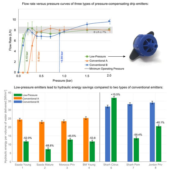
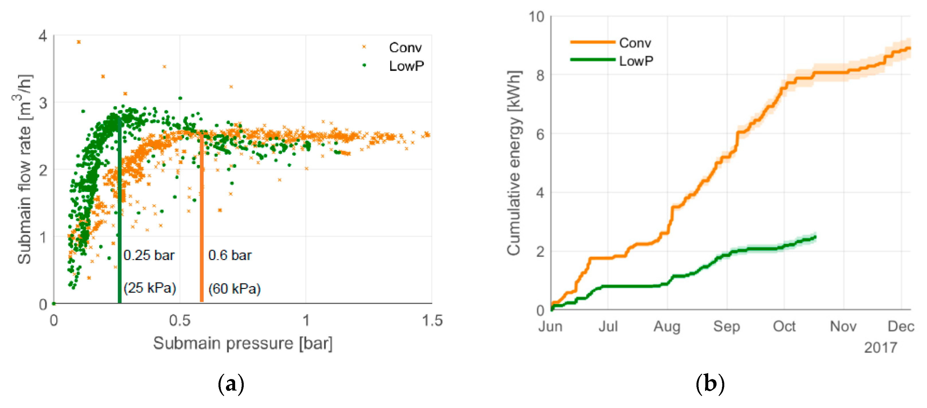
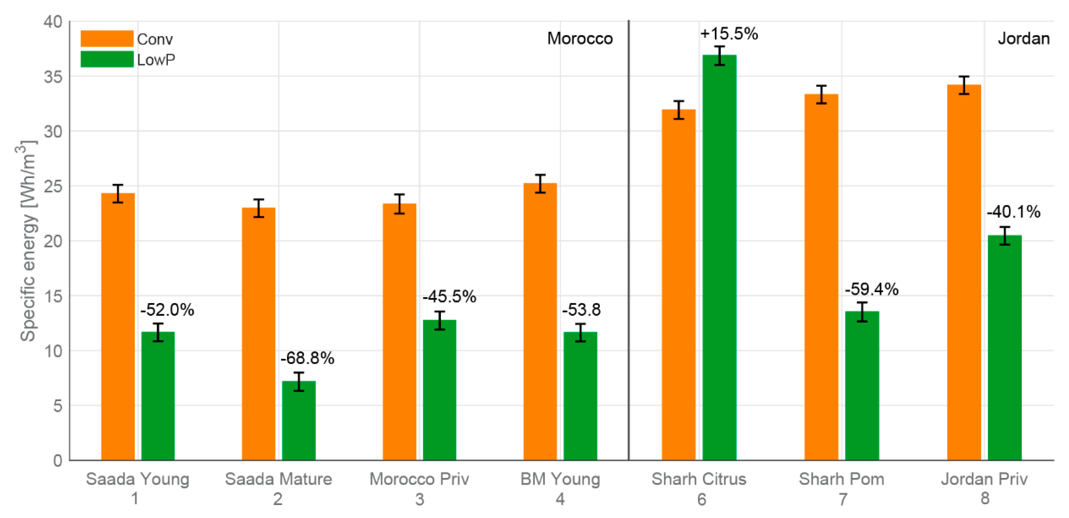
3.1. Flow, Pressure, and Hydraulic Energy

Pressures and flow rates in the submains were measured at seven experimental sites, on two plots (low-pressure and conventional) at each site. These values were used to calculate the specific hydraulic energy needed to deliver a volume of water to each field. In the results below, only irrigation events that passed the cleaning and filtering criteria of Section 2.6 are included (i.e., the pressure setpoint was above the minimum required by the emitters, and pressure and flow sensor data were available). Due to the differences in the number of irrigation events that passed these criteria at each plot, the hydraulic energy results are normalized by the volume of water delivered to the plot (Equation (4)). Below, we point out some notable features from sensor data, describe reasons that led to filtering out certain irrigation events, and summarize the specific energy results for all plots.
Figure 5a,b show an example of the flow and pressure data recorded with submain sensors and filtered according to Section 2.6 for site 7, Sharhabeel Research Station with pomegranate trees, for the full data recording time period. Each spike in the plot represents an irrigation event. The data gap for the conventional emitters between November 13 and December 3 was due to clogging of that flow sensor; other gaps were due to the filtration criteria. During the season, 48 out of 73 (for low-pressure emitters) and 28 out of 82 (for conventional emitters) recorded irrigation events passed the filtration criteria described in Section 2.6, i.e., the mean submain pressure during those events was above 80% of the minimum pressure setting (pset). A larger number of irrigation events for the conventional plot were filtered out, because the higher pressure setting for those emitters was satisfied less often, possibly due to incorrect valve settings or the pump’s outlet pressure decreasing below normal as the level of water in the reservoir decreased, lowering the available net positive suction head. In Figure 5a, this can be seen for the time period August 1–September 10, when all conventional irrigation events were filtered out due to the supplied pressure being too low.
The details of one typical irrigation day from this site are shown in Figure 5c,d. This day featured three irrigation events—two for the conventional emitter plot and one for the low-pressure emitter plot. The low-pressure emitters were able to deliver water at the same flow rate as the conventional emitters, while operating at a submain pressure of 40–60 kPa (0.4–0.6 bar), compared to 100–120 kPa (1.0–1.2 bar) pressure of conventional emitters. This demonstrates their ability to deliver comparable performance at approximately half of the operating pressure. The plot also illustrates the pressure spikes that often occurred at the start of irrigation events.
Figure 6 presents sensor data for site 1, Saada Research Station with young olive trees. Figure 6a illustrates the relationship between flow and pressure for the two plots. Each data point represents a pair of sensor measurements (pressure and flow rate) taken during the season. The data that would otherwise be filtered out are included in this scatter plot to illustrate the effect of operating below the MCIP. As expected from their laboratory characterization (Section 2.4), the low-pressure emitters reach a higher flow rate at lower pressures than conventional emitters. Just above the MCIP of 15 kPa (0.15 bar), the submain flow rate sees a small peak, followed by a decrease towards the regulated flow rate. The conventional emitters begin to pressure-compensate at a higher pressure—around 40–50 kPa (0.4–0.5 bar)—but the regulated flow is more constant.
The consequence of low-pressure emitters providing similar flow rates at lower pressures is lower hydraulic power. When integrated in time over all irrigation events, the cumulative energy needed to pump water for low-pressure emitters increases at a slower pace than that for conventional emitters (Figure 6b). The total hydraulic energy at the end of the irrigation season (Equation (3)) accounts for both pressure and volume of water delivered. Because the water volumes are not always equal between plots being compared, we use specific hydraulic energy—total hydraulic energy normalized by the total volume of water delivered to the plot (Equation (4))—to isolate the effect of the operating pressure for each emitter on pumping energy.
Table 3 summarizes the pressure, flow, and total and specific hydraulic energy results for all experimental sites where sensor measurements were recorded. Overall, plots operating with low-pressure emitters required significantly less hydraulic energy per volume of water delivered than plots with conventional emitters, in both Morocco and Jordan (Figure 7). Sensor data showed that the use of online emitters with low activation pressure led to a reduction in specific hydraulic energy of 43% per plot on average (53% if site 6 is excluded on account of the operating pressure being on average 5.2 times greater than pset—this is further explained below), with a range of 40.1–68.8%. In Morocco, the plots with low-pressure emitters showed reductions in specific energy of 52.0 ± 5.0% at site 1, 68.8 ± 5.6% at site 2, 45.5 ± 5.4% at site 3, and 53.8 ± 4.9% at site 4. In Jordan, the reduction in specific energy for low-pressure emitters compared to conventional emitters was −15.5 ± 3.7% at site 6, 59.4 ± 3.8% at site 7 and 40.1 ± 3.4% at site 8.
The values in Table 3 are based solely on irrigation events that passed the data filtering criteria. At the majority of sites, more events with conventional emitters were filtered out, due to greater difficulty in consistently meeting the higher pressure setting. The difficulty in controlling pressure is evident from the large standard deviation in the mean pressure and values that are often larger than the desired pressure setting, as well as in the example of Figure 6a—the range of pressures it encompasses is a clear indication that the submain pressures diverged significantly from the setpoints when research staff was not present on site to monitor and adjust the pressure. This is especially pronounced for the low-pressure plot on site 6, where the mean pressure was 131 kPa (1.31 bar)—over five times larger than the desired pset of 25 kPa (0.25 bar). The average operating pressure on this plot actually exceeded the operating pressures on the conventional emitter plot, which nullified the energy-saving potential of the low-pressure emitters. At this site, the specific energy for low-pressure emitters was higher, i.e., had negative savings of −15.5 ± 3.7%.
Pressure regulation difficulties occurred because the experimental submains were connected to existing irrigation systems with large pumps meant for irrigating multiple plots at the same time. The pressures to the experimental plots were set using manual valves (pressure-regulating valves for such low pressures were not available), so they may have varied as valves to other plots connected to the same piping network were turned on and off. If each experimental plot had been irrigated independently by a pump sized for its operating pressure setpoint, this variation would have been minimal.

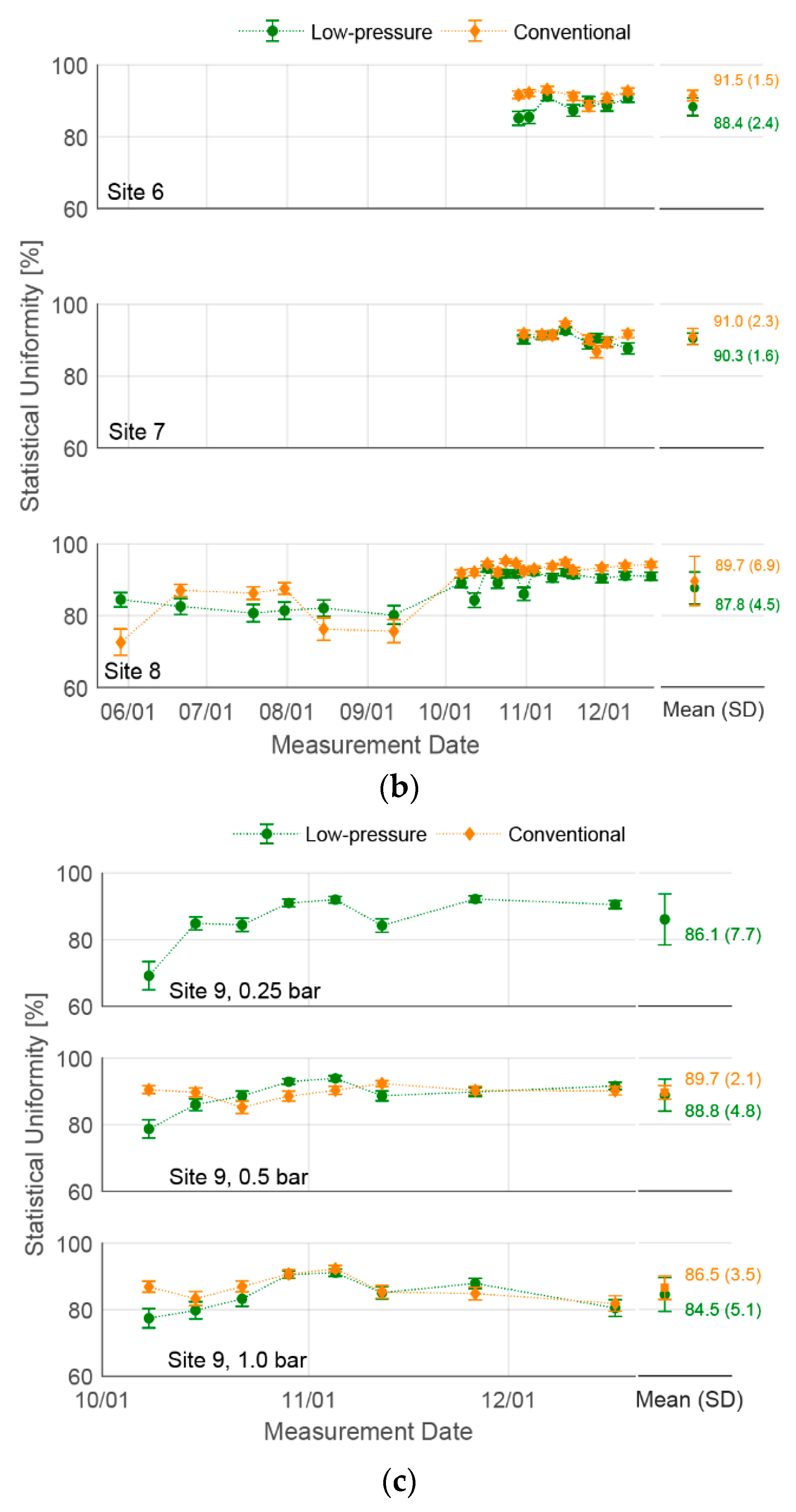
3.2. Uniformity and Clogging

The results of uniformity measurements for low-pressure and conventional emitters, collected following the procedure described in Section 2.5.2, are reported as time series, along with the seasonal averages and standard deviations (Figure 8). In Morocco, the seasonal averages of statistical uniformity were 81–91% for low-pressure emitters and 87–96% for conventional emitters (Figure 8a). Uniformities for both emitter types remained steady over time, with standard deviations below 4% at all plots, except for the conventional emitter plot at Beni Mellal with mature citrus trees (site 5). At this plot, conventional uniformity varied between 73% and 97% throughout the season, with the lowest values occurring between August and October. This reduction in uniformity was attributed to the clogging of emitter outlets by ants and insect larvae. The low-pressure emitters were less affected.
In Jordan, at the freshwater sites, the average statistical uniformities were 88–90% for low-pressure emitters and 89–92% for conventional emitters (Figure 8b). Standard deviations were below 3% for sites 6 and 7, but higher for site 8 (5% for low-pressure emitters, 7% for conventional emitters). On that site, the uniformities measured in the first half of the season (before July) are on average lower than those measured in the second half. This is likely due to the research staff being present at more irrigation events in the latter half, thus having greater control over the operating pressure and emitter conditions (prior to that, some emitters were found without membranes, emitting much higher unregulated flow rates).
At the treated wastewater site (site 9), low-pressure and conventional emitters showed very similar uniformity results (Figure 8c). On the plot operating at 100 kPa (1 bar), the statistical uniformity coefficients of low-pressure and conventional emitters were 84% and 86%, respectively. On the plot with 50 kPa (0.5 bar) submain pressure, the uniformities were 88% for low-pressure emitters and 89% for conventional emitters. On the plot operating at 25 kPa (0.25 bar), uniformities for conventional emitters were not measured because that pressure is far outside the emitter specifications; for low-pressure emitters, the average uniformity was 85%. This value was very close to their uniformity at 100 kPa (1 bar), showing that operating at low pressures did not negatively affect emitter performance. The standard deviation at 25 kPa was larger than that at 100 kPa (7%, compared to 5% at 100 kPa), due primarily to the outlier measurement on October 8th. On that day, 6 of the 32 measured emitters were found to be significantly clogged, and were replaced with new ones after the measurement.
These results show that under typical maintenance procedures, the low-pressure emitters retained uniformity in the “Good” (80–90%) to “Excellent” (90–100%) range, as classified by the American Society of Agricultural Engineering [22] and Bralts [24]. When averaged over all measurements, their uniformities were lower than those of conventional emitters by 7.2% in Morocco and 1.5% in Jordan.

4. Discussion

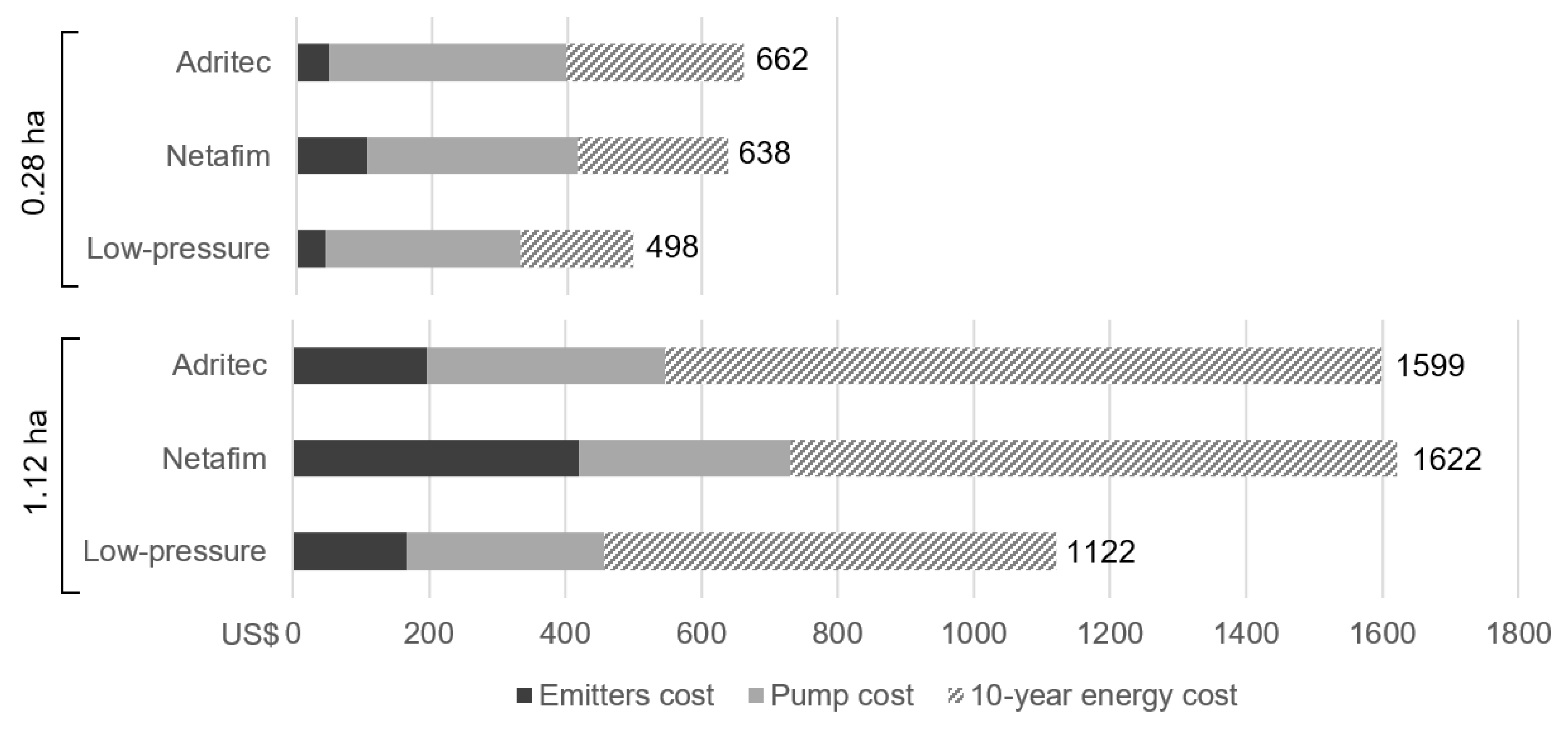
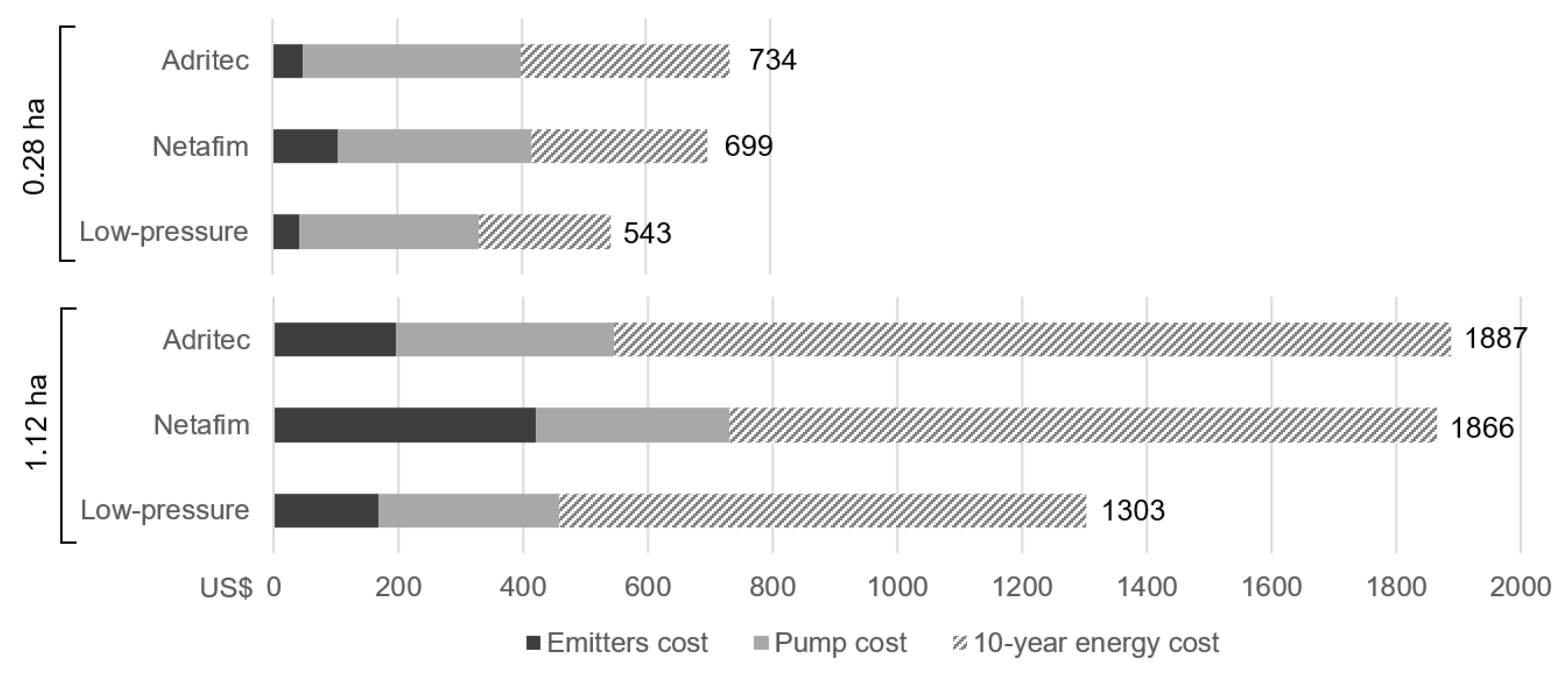
4.1. Energy and Cost Savings

In order to translate the savings in hydraulic energy due to the use of low-pressure emitters, as reported in Section 3.1, into pumping energy cost savings that a farmer might experience, the hydraulic energy needs to be divided by the efficiency of the pump supplying the water. A case study model was used to assess the impact of low-pressure emitters on pumping energy and cost over the course of an irrigation season and to calculate the simple payback period of switching to low-pressure emitters.
A model of a drip irrigation hydraulic network based on one of the experimental plots (Sharhabeel pomegranates, conventional plot) was created in MATLAB [26]. The model is described briefly below; further details on the algorithm of the hydraulic and agronomic models can be found in Appendix C and Ref. [27].
The model uses inputs of pipe geometries (lengths, inner diameters), crop spacing, and emitter flow rate-pressure curves, and calculates flow rates and pressure losses through every segment of the piping network. Pressure losses in network segments are calculated using the Darcy-Weisbach equation. Losses in the filters, valves, and fertigation system are assumed constant and equal to 70 kPa (0.7 bar), based on measurements from field sites. The model outputs a system curve showing the relationship between inlet pressure (i.e., the pressure at the outlet of the pump) and total flow in the drip irrigation network. The system curve is subsequently coupled to a specified pump curve, and their intersection is assumed to be the pump’s operating point. The pump’s efficiency and power are extracted for this operating point and considered to be constant at these values whenever the pump is operational (i.e., transient flows during pump start-up and shut-down are not simulated).
The time of pump operation over the course of an irrigation season is estimated based on the water requirement of the crop at the case study plot (pomegranates). The water requirement (i.e., the crop evapotranspiration) is dependent on the crop type and local weather. This case study uses a typical meteorological year weather file for Irbid, Jordan [28]. Crop evapotranspiration is calculated by multiplying the reference evapotranspiration from the Penman-Monteith equation [29] by the crop coefficient for pomegranates [30].
The total annual pumping energy is equal to the product of the pump power at its operating point and the time period of pump operation over the course of the irrigation season. Each emitter type was simulated with a different model of pump of appropriate capacity, selected such that the operating point was at the pressure required for all emitters to operate just above their MCIP. The three pump models were selected from Pentax CS and CH centrifugal pump models and have similar efficiencies (40%) at the operating points. The pump curves were supplied by the manufacturer [31,32].
Three cases were simulated, each with a different emitter type and corresponding pump (Table 4). Only the capital costs of emitters, pumps, and the operating electricity cost are included in the comparison. The capital costs of all other system components are expected to remain constant across emitter types, because the same submain pipes, filters, and laterals can be used with any of the emitters. The labor cost of installation and system maintenance is also expected to be constant, because the installation process is identical and the clogging rates did not vary significantly between emitters. In order to assess the annual energy costs and the simple payback period of switching to low-pressure emitters, the electricity cost for the pump was assumed to be 0.084 US$/kWh in Jordan [33] and 0.107 US$/kWh in Morocco. The prices of conventional emitters were taken from contractors who purchased and installed them in both locations. The price of the low-pressure emitters was set equal to the selling price of analogous online PC emitters of the same flow rate sold by Jain Irrigation Ltd. in the Indian market, since the low-pressure emitters are not yet commercially sold. This price is expected to be accurate, because the low-pressure emitters are made of the same plastic materials in the same volume as the emitters currently manufactured and sold by Jain Irrigation Ltd. Pump prices were estimates from contractors in Jordan based on pump capacity. Prices for other system components are assumed to be the same for all three scenarios and thus not included in the analysis.
Figure 9 shows a comparison of capital costs for the emitters and pump and 10-year pumping electricity costs (using Jordanian tariffs) for the three scenarios, based on irrigating the example plot of 0.28 ha. For larger farms, one pump would take turns irrigating multiple plots throughout the day; the costs for a larger 1.12-ha farm with four such plots irrigated in sequence are shown in Figure 9 as well. Low-pressure emitters operated with a 1.1-kW pump use 25.6% less pumping energy than emitters A with a 1.5-kW pump and 37.0% less pumping energy than emitters B with a 2.2-kW pump. For the 0.28 ha plot, the total capital and energy cost savings over 10 years are US$140 over a system using emitters A, and $164 over one using emitters B. For the 1.12-ha plot, the total cost savings are $500 over a system with emitters A and $477 over emitters B. Results with Moroccan electricity tariffs are included in Appendix B Figure A3.
For the 1.12-ha farm, these cost savings may be significant enough to warrant retrofitting an existing irrigation system that uses conventional drip emitters with 100 kPa (1.0 bar) MCIP to one that uses low-pressure emitters and a smaller pump. The simple payback period (capital cost for the new pump and emitters divided by the annual energy cost savings) for this switch is 9.2 years in Morocco and 11.8 years in Jordan, based on their respective electricity tariffs. For the small plot of 0.28 ha, the simple payback is significantly longer—26.8 and 34.1 years in Morocco and Jordan, respectively—indicating that a retrofit may not be cost-effective for plots less than 1 ha in area. However, when installing a new drip irrigation system or replacing an existing system at the end of its useful life, low-pressure emitters offer the farmer a way to save on both capital cost and recurring electricity cost. For an off-grid irrigation system, this can translate to additional cost savings on photovoltaic panels.

4.2. Uniformity and Clogging

Although low-pressure emitters remained in the “Good” to “Excellent” range per standard industry classification [22], they showed on average slightly lower uniformity than both sets of conventional emitters. The analysis below shows that this can be attributed primarily to the manufacturing coefficient of variation ( C V m ). The C V m is an indication of the variability of emitter performance due to small variations in the manufacturing process and is calculated per ISO Standard 9261:2004 [21] as
C V m = S q q ¯ × 100 % ,
where q ¯ is the mean flow rate (L/h) and S q is the standard deviation (L/h) of flows for the sample emitters, measured at each test pressure.
The manufacturing coefficient of variation was measured in the lab for the three types of emitters used in the field trials, using a random sample of 25 emitters per type (Figure 10). The low-pressure emitters had C V m in the range of 11.0–15.1% under 70 kPa (0.7 bar); it decreased to below 6% at higher pressures. This was higher than the C V m of the other two emitter types, which ranged between 2.5% and 7.8% in the tested range. The high C V m of emitters A at 30 kPa (0.3 bar) ( C V m = 57 % ; not shown in Figure 10) is due to the non-leakage function, which prevents flow below a shut-off pressure. This shut-off pressure is not exactly the same for all emitters, which leads to a high standard deviation with a low mean flow rate. At pressures below 20 kPa (0.2 bar), the C V m for emitters A was undefined, as the tested emitters showed zero flow.
Statistical Uniformity ( S U ) measured in the field can be related to manufacturing and other coefficients of variation as follows:
S U = 1 C V f i e l d = 1 C V m 2 + C V h y d 2 + C V c l o g 2 ,
where C V f i e l d is the measured coefficient of flow variation in the field due to all factors, C V h y d is the flow variation due to hydraulic pressure variations, C V c l o g is the flow variation due to clogging, and the three sources of variation are assumed to be uncorrelated [23,35]. Assuming that all emitters are operating above their MCIPs and clogging is negligible, the last two terms under the square root would be zero and uniformity would be a function of C V m only.
At the operating pressures of 30–40 kPa (0.3–0.4 bar), the low-pressure emitters have C V m of 15 ± 2%, which translates to a statistical uniformity of 85 ± 2% when hydraulic and clogging variation is negligible. Actual uniformity for low-pressure emitters, averaged over all sites and measurements, was comparable to this estimate: 87 ± 5%. Conventional emitters, on the other hand, have C V m in the 3–7% range at their operating pressures, implying a statistical uniformity of 93–97% when hydraulic and clogging variation is neglected. This explains the slightly higher measured SUs for conventional plots (90 ± 5% for emitters B in Jordan; 93 ± 6% for emitters A in Morocco). These measurements and standard deviations indicate that clogging did not play a significant role in field uniformity when standard maintenance procedures were followed (Section 2.5.2; Appendix A.1). Furthermore, there was no significant difference in field uniformity between sites with severe and moderate water clogging potentials.
Another possible source of emitter flow variation is changes in ambient air and water temperature. Elevated temperatures may lead to slight thermal expansion of the emitter materials, especially the elastomeric membrane responsible for the pressure-compensating function, thus affecting the water flow path. For example, Oliver et al. [36] measured the performance of three types of inline PC emitters under heating and cooling cycles, and observed a trend of slightly decreasing flows and higher CVs at higher temperatures (above 23 °C). In the present field experiments, thermal effects were not monitored, but would warrant further study in laboratory conditions, as they may affect low-pressure and conventional emitters differently due to differences in their membrane properties.
While measured uniformities for low-pressure emitters were considered good, there are several ways to improve it further. First, the manufacturing process should be more closely controlled to ensure tight tolerances, especially in the mold-making and injection molding stages. Additional variation may be due to differences in torque with which the emitter cap is screwed on to the emitter body during the assembly stage. To address this, assembly could be automated instead of being done manually, or additional features could be added to the outside of the emitter body that would prevent screwing on the cap beyond a certain limit.
Second, effective variation in the field can be reduced by using multiple emitters per crop. Assuming C V m is due to random variation, using multiple emitters per crop leads to positive and negative deviations from mean flow canceling each other out. The S U per crop (rather than per emitter) can then be calculated as:
S U c r o p = 1 1 S U n ,
where n is the number of emitters per crop [23]. The experimental sites used between 4 and 12 emitters per tree, depending on species and age. Adjusting the average measured S U for low-pressure emitters (87%) by the number of emitters per tree results in effective S U c r o p values from 93.5% for 4 emitters per crop to 96.3% for 12 emitters per crop. A plot relating the number of emitters per crop to the increase in effective crop uniformity can be seen in Appendix B Figure A4.

5. Conclusions

A new design of online pressure-compensating drip emitters, with MCIP of 15 kPa (0.15 bar), was manufactured and tested on farms in Morocco and Jordan during the 2017 irrigation season. A total of 5696 low-pressure emitters were initially installed; of these, 640 emitters were used on a site using treated wastewater in Jordan, and the rest were installed on sites with diverse sources of freshwater. At the freshwater sites, the low-pressure emitters reduced the hydraulic energy per volume of water delivered for irrigation by 53% on average, compared to commercial online emitters with higher compensating pressures of 50 and 100 kPa (0.5 and 1.0 bar). When maintained according to standard practices, the low-pressure emitters demonstrated consistently good uniformity throughout the season with water of moderate and severe clogging potential. Their average field uniformity was 87%, primarily on account of high manufacturing variation. At the treated wastewater site, low-pressure emitters showed good uniformity that was independent of the pressure at which they were operating (25, 50, and 100 kPa, or 0.25, 0.5, and 1.0 bar) and comparable to that of commercial emitters at the higher pressures of 50 and 100 kPa (0.5 and 1.0 bar).
Study results demonstrate the value of using low-pressure online emitters and show that they can act as good substitutes to commercial online emitters, while maintaining the same price point due to a similar manufacturing process with the same materials. Based on an analysis of typical 0.28-hectare and 1.12-hectare drip irrigation systems with pumps powered by electricity, low-pressure emitters can lead to a 22–31% reduction in the capital cost of the pump and emitters and the 10-year energy cost, due to the lower-capacity pump required. The energy use reduction offers environmental benefits in the form of reduced greenhouse gas emissions from electricity generation. The reduced capital cost and capacity of the pump may encourage more farmers to install off-grid solar-pumped drip systems, a fully renewable alternative to grid electricity or diesel fuel. This could be especially beneficial to small farmers in remote areas that do not have consistent access to electricity or fuel, allowing them to produce higher crop yields through consistent irrigation. In addition to electricity reduction of pumped systems, low-pressure emitters can enable wider use of gravity-fed drip systems in regions with elevated water sources.
Further work on emitter design and manufacturing is warranted, such as a dimensional sensitivity analysis and an examination of the manufacturing process in order to reduce the manufacturing coefficient of variation, to enable higher uniformity. A targeted study of emitter clogging, with identification of features that are most likely to cause clogging, may inspire more improvements to the current design. In order to increase their versatility, a suite of low-pressure online emitters with different flow rates should be developed and manufactured following the same process as the 8 L/h emitters that were used in this trial. The development of low-pressure PC emitters may drive further research into reducing energy used by drip irrigation systems and help make drip irrigation systems more sustainable and affordable to farmers.

Author Contributions

Conceptualization, A.G.W., S.A., V.N., S.T.; methodology, S.A., J.S., E.B., G.M., V.N., S.T.; software, J.S.; validation, J.S., S.A.; formal analysis, J.S.; investigation, K.A.N., K.B.M., B.B., A.B. (Abdelaziz Bouizgaren), L.S.; resources, A.B. (Abdeljabar Bahri), N.M., R.M.; data curation, G.M., E.B., J.S.; writing—original draft preparation, J.S.; writing—review and editing, J.S., S.A., G.M., V.N., S.T., B.B., N.M., A.G.W.; visualization, J.S.; supervision, V.N., S.T.; project administration, S.A., N.M., A.B. (Abdeljabar Bahri), R.M., G.M., V.N., S.T.; funding acquisition, A.G.W., V.N., S.T.

Funding

This study was supported by USAID Cooperative Agreement Number AID-OAA-A-16-00055 (BAA-MWSI-ME-2015).

Acknowledgments

The authors would like to thank Jain Irrigation Ltd. for manufacturing and conducting preliminary testing on prototype emitters. The authors are grateful to the National Agricultural Research Center (NARC) in Jordan, the Institut National de la Recherche Agronomique (INRA) in Morocco, and the private farmers in Morocco and Jordan who provided access to their farms for these experiments. Sally Beiruti and Tristan MacLaurin assisted with laboratory measurements.

Conflicts of Interest

The authors declare no conflict of interest.

Appendix A. Supplementary Methods

Appendix A.1. Irrigation System Maintenance at Experimental Sites

Sites measuring emitter performance with freshwater: Depending on the site, sand and disk filters were cleaned every 2 weeks (Saada, Moroccan private farm) or when the pressure drop through the filters surpassed 50 kPa (0.5 bar) (Beni Mellal). Sand filters were cleaned by backwashing the filters for approximately 15 min. Disk filters were cleaned by removing the filter from its housing, disassembling the disks, soaking in an acid solution, and washing with a water jet. System pipes were flushed every 2–4 weeks by removing submain and lateral caps and pumping high-velocity water through the system until the water exiting the pipes was visibly clear. At Sharhabeel, after clogging with algae was noticed on October 3, 2017, acid injection was performed every 2 weeks until the end of the season, by mixing a 2% phosphoric acid solution in the fertilizer tank and pumping the entire volume through the system.
Site measuring emitter performance with treated wastewater: System maintenance consisted of filter disk cleaning when the pressure drop through the filters became too high to deliver the required 100 kPa (1 bar) pressure at the submain. This typically required cleaning the disk filter after every irrigation event by soaking it in chlorine for 3 h. The sand filter was cleaned by replacing the sand every 2 months.

Appendix A.2. Pressure and Flow Sensor Calibration

Pressure sensors were calibrated using a Fluke 718 pressure calibrator (Fluke, Everett, WA, USA, ±0.3 kPa). Flow sensors (DFMT-25A, Dwyer, Michigan City, IN, USA on sites 1 and 5; PFT, Dwyer, Michigan City, IN, USA on sites 2–3, 6–9) were calibrated to locally-purchased analog flow totalizers installed on the same pipe: Woltman LXLGC 15 m3/h (Shanxi Solid Industrial Co., Taiyuan, Shanxi, China, ±2%) on site 2, Hidroconta 15 m3/h (Hidroconta, Murcia, Spain, ±2%) on site 3, Woltman 15 m3/h (Shanxi Solid Industrial Co., Taiyuan, Shanxi, China, ±2%) on site 5, and Sanlian LXSG-40E 10 m3/h (Sanlian Water Meter Co., Fenghua, Zhejiang, China, ±2%) on sites 6–9. On site 1, the totalizers were oversized for the submain flow rate so their accuracies could not be determined; hence, the flow sensors (DFMT-25A, Dwyer, Michigan City, IN, USA, ±0.017 m3/h) were used without additional field calibration at this site. Several flow sensors of model PFT (Dwyer, Michigan City, IN, USA) were cleaned and recalibrated as needed when sensor operation was inhibited by clogging or corrosion.

Appendix B. Supplementary Tables and Figures

Figure A1. General site diagram, highlighting one control-test pair of plots. Water was delivered to both plots by the same pump, via a main pipe that branched into multiple submain pipes. The instrumentation sections on the submains contained a valve to regulate pressure, and flow and pressure sensors to monitor the water flow.
Water 11 01195 g0a1
Figure A2. Site diagram for the treated wastewater site (Ramtha Research Station) in Jordan. A pressure-regulating valve at the start of each submain was used to set a different pressure for each: 25, 50, and 100 kPa (0.25, 0.5, and 1 bar). The submains at 50 and 100 kPa (0.5 and 1 bar) delivered water to 16 laterals each—8 with low-pressure emitters, 8 with conventional emitters. The submain at 25 kPa (0.25 bar) delivered water to 16 laterals with low-pressure emitters only, because it was far below the recommended operating pressure for conventional emitters.
Water 11 01195 g0a2
Figure A3. Capital costs for emitters and pumps, and energy costs for a 10-year operational period for the example field (0.28 ha, pomegranate crop, 700 emitters with 8 L/h rated flow rate) and a larger 1.12-ha farm with four plots of that size, irrigated in sequence. Costs in US$ are shown for the three types of emitters, for the pumps required to operate with all emitters above their MCIP and for electricity over a 10-year period.
Water 11 01195 g0a3
Figure A4. Effective statistical uniformity per crop when it is watered by multiple emitters with a certain C V m . Assuming C V m is due to random variation, positive and negative deviations from the mean flow rate of individual emitters cancel each other out, resulting in higher effective uniformity. The starting point of this plot is the average measured field statistical uniformity for a single low-pressure emitter.
Water 11 01195 g0a4

Appendix C. Drip Irrigation System Model Description

A model of the agronomy and hydraulics of a drip irrigation system was programmed in MATLAB [26].

Hydraulics Module

The hydraulics module calculates the pressure-flow curve for the hydraulic system consisting of a main pipe, submain pipe, and lateral pipes with emitters. The module assumes that water at a specific pressure head p s y s is input from a pump into one main pipe. The start of the main pipe includes several pressure losses due to components usually installed after the pump—filters, valves, and fertigation equipment. These are assumed to be constant and equal to 70 kPa (0.7 bar), based on measurements from field sites. After the pump house components, the main pipe conveys water to one or more submains. Each submain delivers water to multiple laterals that branch off from the submain. Each lateral has a number of drip emitters, assumed to be equally spaced.
For each pipe, inner diameter, roughness, and the spacing of smaller pipes or emitters connected to the pipe are specified. Major pressure losses in each pipe segment (i.e., straight length of pipe between any inlets/outlets or minor loss locations) of length L and inner diameter D are calculated using the Darcy-Weisbach equation (Equation (A1)). Minor pressure losses are modeled for tee fittings at the start of each pipe branching off from a larger pipe (Equation (A2)), where K = 1 for tee losses in branch flow [37]. Minor losses for water flowing over an emitter are neglected.
Δ p m a j o r = f d L D ρ V 2 2
Δ p m i n o r = K ρ V 2 2
Here, ρ is the fluid density (kg/m3), V is the average velocity of the fluid in this pipe segment (m/s), L and D are the pipe segment length (m) and inner diameter (m), respectively, and f d is the Darcy friction factor. For f d in laminar flow, Equation (A3) applies; in turbulent flow, the Swamee-Jain formula is used (Equation (A4)) [38].
f d = 64 R e   for   R e < 2300
f d = 0.25 [ l o g 10 ( ε 3.7 D + 5.74 R e 0.9 ) ] 2   for   R e 2300
R e = ρ V D μ is the Reynolds number in the pipe segment, μ is the fluid dynamic viscosity (Pa∙s), and ε is the pipe roughness (m).
At each node where pipe segments connect, mass conservation is assumed. The total flow in the system at a given p s y s is governed by the outflow from the drip emitters. For a pressure-compensating emitter with minimum compensating inlet pressure (MCIP) p m c i p (Pa), flow Q out of the emitter is modeled as linear Q = k p p m c i p when 0 < p < p m c i p , and as following the curve Q = k p x when p p m c i p . Here, p is the water pressure at the emitter inlet (Pa), k is the flow coefficient (m/s or m/s/Pax), and x is the pressure compensation exponent. k and x are constants determined by the design of the emitter. For a perfect pressure-compensating emitter, x ≈ 0 and the emitter flow Q is constant above the MCIP.
The calculation of flow and pressures at every point in the system is performed iteratively, because the pressure losses depend on the fluid velocity. For a given p s y s , all emitter flow rates are initialized to their rated flow, then system pressures are re-calculated using the initialized flows, and the iterations are repeated until convergence in flow rates occurs, with a maximum convergence error of 1 L/h for total flow entering any submain. This calculation is run for a vector of input pressures p ¯ s y s , generating a system curve of system flow rates Q ¯ s y s versus pressures.
The point on the curve where the system will operate when a selected pump is connected to it will depend on where it intersects the pump’s pressure-flow curve. The electrical power needed to run the pump at this operating point P p u m p (W) is calculated from the pressure p p u m p (Pa), flow Q p u m p (m3/s), and pump’s efficiency η at the operating point (Equation (A5)). The pump’s efficiency and power are considered to be constant at the operating point whenever the pump is operational, i.e., transient flows during pump start-up and shut-down are not simulated.
P p u m p = p p u m p Q p u m p η

Agronomy Module

The agronomy module calculates the crop water requirement (i.e., the crop evapotranspiration, E T c ) based on local weather data and the selected crop. The crop water requirement is computed on a daily basis using the method presented in Irrigation and Drainage Paper 56 by the Food and Agriculture Organization of the United Nations (FAO) [29]. First, the Penman-Monteith equation (Equation (A6)) is used to calculate the reference evapotranspiration E T 0 based on meteorological data:
E T 0 = 0.408 Δ ( R n e t G ) + γ C T + 273 u 2 ( e s e a ) Δ + γ ( 1 + 0.34 u 2 )
where E T 0 is the reference evapotranspiration (mm/day) for a grass reference crop of 0.12 m height; R n e t is the net radiation at the crop surface (MJ/m2/day); G is the soil heat flux density (MJ/m2 day), assumed 0 for daily intervals; T is the daily average air temperature at 2 m height (°C); u 2 is the daily average wind speed at 2 m height (m/s); e s is the saturation vapor pressure (kPa) at air temperature T; e a is the actual vapor pressure (kPa) at air temperature T; Δ is the slope of vapor pressure curve (kPa/°C) at air temperature T; C = 900 is the time step constant for daily intervals; and γ is the psychrometric constant (kPa/°C), equal to 0.665 × 10 3 × P , where P is the atmospheric pressure (kPa). Vapor pressure and the slope of vapor pressure curve are computed using minimum and maximum hourly temperatures and relative humidity levels recorded throughout the day. Further details of the calculations of specific terms in the Penman-Monteith equation can be found in Ref. [29]. In this paper’s case studies, meteorological variables are extracted from typical meteorological year weather files (ASHRAE IWEC2), containing representative hourly average temperature, humidity, and radiation values for a given location over the past 20 years.
Once the reference evapotranspiration is calculated, it is scaled to the crop-specific evapotranspiration ( E T c ) using the single crop coefficient model ( K c ):
E T c = K c E T 0 ,
where K c is a function of the crop and the stage in the crop’s development. A crop database was constructed from data in Ref. [29], with lengths of development stages in days and K c values corresponding to each stage ( K c , i n i , K c , m i d , K c , e n d ). Initial and mid-season stages have constant coefficients ( K c , i n i and K c , m i d ), with a linear change in coefficient during the crop development stage (between K c , i n i and K c , m i d ) and late season (between K c , m i d and K c , e n d ). When climate conditions are different from the climates used for tabulated Kc values (climates where average R H m i n , m e a n ≠ 45% or u 2 , m e a n ≠ 2.0 m/s), K c , m i d and K c , e n d are adjusted per the equation below, provided that the tabulated value of K c , e n d   ( T a b ) ≥ 0.45:
K c , m i d / e n d = K c , m i d / e n d   ( T a b ) + ( 0.04 ( u 2 , m e a n 2 ) 0.004 ( R H m i n , m e a n 45 ) ) ( h 3 ) 0.3 ,
where K c , m i d / e n d   ( T a b ) is the tabulated value for K c , m i d or K c , e n d , h is the mean plant height during the mid/late-season stage (m) (tabulated), and mean values of u 2 , m e a n and R H m i n , m e a n are calculated for the corresponding growth stage from the weather data.
After E T c is calculated for the given crop in mm/day, it is converted to the volume of water that needs to be delivered to each subunit in the field. A subunit is defined as an area irrigated by one submain with its connected laterals. For a subunit with a given area A s u b (m2), the water volume V s u b (m3/day) is calculated as:
V s u b = f w A s u b E T c / 1000 ,
where f w is the soil wetted fraction, which is assumed to be 0.3 for drip irrigation [29].

System Operating Time and Cost Module

The water requirement from the agronomy module V s u b (m3/day) and the operating point of the pump from the hydraulics module Q p u m p (m3/s) are combined to compute the time of pump operation t p u m p (s) over the course of a growing season of a crop:
t p u m p = i = 1 n V s u b , i Q p u m p
where V s u b , i is the volume of water (m3/day) delivered to the field on day i = 1 , , n of a growing season consisting of n days. From the pump power at its operating point P p u m p (W), the total annual energy to run the pump E p u m p (J) can be calculated as:
E p u m p = P p u m p t p u m p
Unit costs of the pump ( C p ), emitters ( C e ) in US$, the total number of emitters ( n e ), and the electricity ( C k W h ) in US$ per kWh, are used to calculate the capital cost of the pump and emitter combination ( C c a p ), the operating cost over a number of years n y ( C o p e r ) (Equations (A12) and (A13)). In this comparison study, maintenance costs or costs of the piping network are not considered as they are assumed to remain constant when switching between conventional and low-pressure emitters.
C c a p = C p + C e n e
C o p e r = n y C k W h E p u m p 3.6 × 10 6

References

  1. FAO (Food and Agriculture Organization of the United Nations). The State of Food and Agriculture: Leveraging Food Systems for Inclusive Rural Transformation; FAO: Rome, Italy, 2017. [Google Scholar]
  2. Postel, S.; Polak, P.; Gonzales, F.; Keller, J. Drip irrigation for small farmers: A new initiative to alleviate hunger and poverty. Water Int. 2001, 26, 3–13. [Google Scholar] [CrossRef]
  3. Wang, X.; Huo, Z.; Guan, H.; Guo, P.; Qu, Z. Drip irrigation enhances shallow groundwater contribution to crop water consumption in an arid area. Hydrol. Process. 2018, 32, 747–758. [Google Scholar] [CrossRef]
  4. Narayanamoorthy, A. State of Adoption of Drip Irrigation for Crops Cultivation in Maharashtra. In Micro Irrigation Systems in India; Viswanathan, P., Kumar, M., Narayanamoorthy, A., Eds.; India Studies in Business and Economics; Springer: Singapore, 2016. [Google Scholar]
  5. Ibragimov, N.; Evett, S.R.; Esanbekov, Y.; Kamilov, B.S.; Mirzaev, L.; Lamers, J.P.A. Water use efficiency of irrigated cotton in Uzbekistan under drip and furrow irrigation. Agric. Water Manag. 2007, 90, 112–120. [Google Scholar] [CrossRef]
  6. ICID (International Commission on Irrigation and Drainage). Agricultural Water Management for Sustainable Rural Development: Annual Report 2016–2017; ICID: New Delhi, India, 2017. [Google Scholar]
  7. Shamshery, P.; Winter, A.G. Shape and form optimization of on-line pressure-compensating drip emitters to achieve lower activation pressure. J. Mech. Des. 2018, 140, 035001. [Google Scholar] [CrossRef]
  8. Shamshery, P.; Wang, R.-Q.; Tran, D.V.; Winter, A.G. Modeling the future of irrigation: A parametric description of pressure compensating drip irrigation emitter performance. PLoS ONE 2017, 12, e0175241. [Google Scholar] [CrossRef] [PubMed]
  9. Joffé, G. The Impending Water Crisis in the MENA Region. Int. Spect. 2016, 51, 55–66. [Google Scholar] [CrossRef]
  10. Tekken, V.; Costa, L.; Kropp, J.P. Increasing pressure, declining water and climate change in north-eastern Morocco. J. Coast. Conserv. 2013, 17, 379–388. [Google Scholar] [CrossRef]
  11. Alaoui, M. Water sector in Morocco: Situation and perspectives. J. Water Resour. Ocean Sci. 2013, 2, 108–114. [Google Scholar]
  12. Berrada, A. Assessment of Drip Irrigation in Morocco with Particular Emphasis on the Plain of Tadla; Colorado State University: Fort Collins, CO, USA, 2009. [Google Scholar]
  13. Kalpakian, J.; Legrouri, A.; Ejekki, F.; Doudou, K.; Ouardaoui, A.; Kettani, D. Obstacles facing the diffusion of drip irrigation technology in the Middle Atlas region of Morocco. Int. J. Environ. Stud. 2014, 71, 63–75. [Google Scholar] [CrossRef]
  14. MAPM (Ministry of Agriculture, Fisheries, Rural Development, Water and Forests). Maroc Vert. Available online: http://www.agriculture.gov.ma/en/pages/strategy (accessed on 24 January 2017).
  15. FAO. AQUASTAT Country Fact Sheet: Jordan. Available online: http://www.fao.org/nr/water/aquastat/ data/cf/readPdf.html?f=JOR-CF_eng.pdf (accessed on 1 July 2018).
  16. Ministry of Water and Irrigation. Jordan Water Sector Facts & Figures; Ministry of Water and Irrigation: Amman, Jordan, 2015.
  17. USAID (United States Agency for International Development). Water Resources and Environment. Available online: https://www.usaid.gov/jordan/water-and-wastewater-infrastructure (accessed on 1 July 2018).
  18. Nakayama, F.S.; Bucks, D.A. Water quality in drip/trickle irrigation: A review. Irrig. Sci. 1991, 12, 187–192. [Google Scholar] [CrossRef]
  19. Harris, I.; Jones, P.D.; Osborn, T.J.; Lister, D.H. Updated high-resolution grids of monthly climatic observations—The CRU TS3.10 Dataset. Int. J. Climatol. 2014, 34, 623–642. [Google Scholar] [CrossRef]
  20. Meteorological Department of Jordan. Sharhabeel (Wadi El-Rayyan) and Ramtha Stations; Meteorological Department of Jordan: Amman, Jordan, 2019.
  21. ISO (International Organization for Standardization). ISO Standard 9261:2004(E), Agricultural Irrigation Equipment—Emitters and Emitting Pipe—Specification and Test Methods; ISO: Geneva, Switzerland, 2004. [Google Scholar]
  22. Lamm, F.R.; Storlie, C.A.; Pitts, D.J. Revision of EP458: Field evaluation of microirrigation systems. In Proceedings of the ASAE Annual International Meeting, American Society of Agricultural Engineers, Minneapolis, MN, USA, 10–14 August 1997. [Google Scholar]
  23. Bralts, V.F.; Wu, I.-P.; Gitlin, H. Drip Irrigation Uniformity Considering Emitter Plugging. Trans. ASAE 1981, 24, 1234–1240. [Google Scholar] [CrossRef]
  24. Bralts, V.F. Field Performance and Evaluation. In Trickle Irrigation for Crop Production: Design, Operation, and Management; American Society of Agricultural Engineers: St. Joseph, MI, USA, 1986; pp. 216–240. [Google Scholar]
  25. United States Salinity Laboratory Staff. Diagnosis and Improvement of Saline and Alkali Soils; US Department of Agriculture: Washington, DC, USA, 1954.
  26. MathWorks, Inc. MATLAB R2017b. 2017. Available online: https://www.mathworks.com/products/matlab.html (accessed on 1 January 2017).
  27. Sokol, J.; Sheline, C.; Grant, F.; Winter, A.G. Development of a System Model for Low-Cost, Solar-Powered Drip Irrigation Systems in the MENA Region. In Proceedings of the ASME 2018 International Design Engineering Technical Conferences and Computers and Information in Engineering Conference, Quebec City, QC, Canada, 26–29 August 2018; Volume 2B. [Google Scholar]
  28. White Box Technologies. Weather Data for Energy Calculations. Available online: http://weather.whiteboxtechnologies.com (accessed on 1 May 2017).
  29. FAO. Irrigation and Drainage Paper 56: Crop Evapotranspiration-Guidelines for Computing Crop Water Requirements; FAO: Rome, Italy, 1998. [Google Scholar]
  30. NaanDanJain. Pomegranate. Available online: http://naandanjain.com/solutions/pomegrante/ (accessed on 7 August 2018).
  31. Pentax Industries. CH Catalogue. 2018. Available online: https://admin.pentax-pumps.it/WebResource/Pentax/Serie/PdfCatalogo/CH_50HZ.pdf (accessed on 1 July 2018).
  32. Pentax Industries. CS Catalogue. 2018. Available online: https://admin.pentax-pumps.it/WebResource/Pentax/Serie/PdfCatalogo/CS_50HZ.pdf (accessed on 1 July 2018).
  33. NEPCO. Electricity Tariff in Jordan. Available online: http://www.nepco.com.jo/en/ electricity_tariff_en.aspx (accessed on 1 July 2018).
  34. Curto, J.D.; Pinto, J.C. The coefficient of variation asymptotic distribution in the case of non-iid random variables. J. Appl. Stat. 2009, 36, 21–32. [Google Scholar] [CrossRef]
  35. Bralts, V.F.; Wu, I.-P.; Gitlin, H. Manufacturing Variation and Drip Irrigation Uniformity. Trans. ASAE 1981, 24, 113–119. [Google Scholar] [CrossRef]
  36. Oliver, M.M.H.; Hewa, G.A.; Pezzaniti, D. Thermal variation and pressure compensated emitters. Agric. Water Manag. 2016, 176, 29–39. [Google Scholar] [CrossRef]
  37. White, F.M. Fluid Mechanics, 7th ed.; McGraw-Hill: New York, NY, USA, 2003. [Google Scholar]
  38. Swamee, P.K.; Jain, A.K. Explicit equations for pipe flow problems. J. Hydraul. Div. ASCE 1976, 107, 657–664. [Google Scholar]
Figure 1. Relationship between flow rate and water pressure at the emitter inlet for pressure-compensating (PC) emitters. The Minimum Compensating Inlet Pressure (MCIP) is the pressure above which the emitter’s flow rate is within 7% of its nominal flow rate.
Water 11 01195 g001
Figure 2. Locations of experimental sites in (a) Morocco and (b) Jordan (Google Maps, 2018a, 2018b). In Morocco, the sites were located in the Marrakech (1–3) and Beni Mellal (4, 5) regions. In Jordan, the sites were in the Northern Jordan Valley (6, 7), Al-Mafraq (8) and Ramtha (9) regions.
Water 11 01195 g002
Figure 3. (a) Photograph of the low-pressure emitter. (b) Characteristic curves for low-pressure and conventional emitters used in field trials, as measured in lab tests (n = 25 for each type of emitter; mean and standard deviation are plotted). All emitters have a nominal flow rate of 8 L/h, low-pressure emitters have an MCIP of 15 ± 5 kPa (0.15 ± 0.05 bar); emitters A (conventional on Morocco sites) have an MCIP of 40 ± 5 kPa (0.40 ± 0.05 bar) for the PC-NL version; emitters B (conventional on Jordan sites) have an undefined MCIP as the flow does not reach a compensated state, but the minimum pressure above which the flow rate remains equal to or greater than nominal is 95 ± 5 kPa (0.95 ± 0.05 bar).
Water 11 01195 g003
Figure 4. Diagram of a typical experimental site, featuring two plots with low-pressure emitters and conventional emitters as the control (site 6, Sharhabeel Citrus). Each circle represents one citrus tree; the filled-in circles are the 16 trees per plot selected for uniformity measurement. At each of these trees, the flow rates of two emitters were measured for a total of 32 emitters per plot, and the measured flow rates were used to calculate statistical uniformity of water application throughout the plot. The instrumentation section components are shown, including the valves used to set submain pressures, and pressure and flow measurement instruments.
Water 11 01195 g004
Figure 5. Example of submain (a) flow rate, and (c) pressure sensor data collected during the 2017 irrigation season for low-pressure (LowP) and conventional (Conv) emitter plots at the Sharhabeel site with pomegranates. The mean values over the season are shown with dashed lines. Zoom in on one day of sensor data for (b) flow rate and (d) pressure, comprising one irrigation event on the low-pressure emitter plot and two irrigation events on the conventional emitter plot. The low-pressure emitters delivered the same flow rate at a submain pressure of 40–60 kPa (0.4–0.6 bar) as the conventional emitters at a pressure of 100–120 kPa (1.0–1.2 bar).
Water 11 01195 g005
Figure 6. Sensor and calculated specific energy data for site 1 in Morocco. (a) Submain flow rate plotted against submain pressure, for pipes supplying both low-pressure (LowP) and conventional (Conv) emitter plots. All recorded data points are plotted, even for irrigation events with pressures below the MCIP, in order to demonstrate the full performance curve of the two emitters. The setpoint pressures for both submains are indicated with solid lines. (b) Cumulative hydraulic energy over the course of data recording. Only post-filtered data points are included in this plot. Vertical segments represent the increase in energy during an irrigation event; horizontal segments are data gaps or non-irrigated periods when flow rate and pressure are zero. The shaded areas represent the uncertainty due to flow and pressure sensor accuracy.
Water 11 01195 g006
Figure 7. Specific hydraulic energy (total hydraulic energy per total volume of water delivered) at all experimental sites with sensor measurements for conventional (Conv) and low-pressure (LowP) emitters. In all cases, low-pressure emitters used less energy except at the Sharhabeel Citrus site, which had difficulty keeping the operating pressure at the low pressure setting. The percentages represent the change in specific hydraulic energy for low-pressure emitter plots compared to conventional plots.
Water 11 01195 g007
Figure 8. Statistical uniformity (SU) for all experimental plots in (a) Morocco sites (1–5); (b) Jordan freshwater sites (6–8); (c) Jordan wastewater site (9). Time series of uniformity over the season is shown, with the marker representing the measured SU for the sample size of 32 emitters per plot, and the error bars representing the standard error of the measurement. The seasonal means and standard deviations (in parentheses) are shown for each site as well. Low-pressure emitters have uniformities comparable to those of conventional emitters B in Jordan and slightly lower than those of conventional emitters A in Morocco.
Water 11 01195 g008aWater 11 01195 g008b
Figure 9. Capital costs for three emitter types, for the pumps required to operate each emitter type above its MCIP, and pumping electricity costs (using the Jordan tariff) for a 10-year operational period. Results are shown for the example plot (0.28 ha, pomegranate crop, 700 emitters with 8 L/h rated flow rate) and for a larger 1.12-ha farm with four plots of that size, irrigated in sequence.
Water 11 01195 g009
Figure 10. Manufacturing coefficient of variation ( C V m ) of the three types of low-pressure and conventional emitters used in field trials, as measured in lab tests (n = 25 for each type of emitter), computed per Equation (5) for a range of inlet pressures, and plotted with the standard error of CV [34]. The high C V m of emitters A at 30 kPa (0.3 bar) ( C V m = 57 % ; not shown in plot) is due to variation in shut-off pressure for the non-leakage feature, leading to a high standard deviation at a low mean flow rate.
Water 11 01195 g010
Table 1. Climatic conditions and water quality at experimental locations. Water was sampled from the reservoir (pre-filtration) one or more times throughout the 2017 irrigation season; for sites with more than one analysis, the mean of all measurements is listed with the standard deviation. Clogging potential is based on classification by Nakayama [18] using the mean values. Climate parameters are averages from years 1980–2016 [19], except for Beni Mellal Research Station with values averaged from 1970–2007 [12], and Sharhabeel and Ramtha Research Stations with values averaged from 1961–2003 [20].
LocationWeatherWater Quality
CountrySite NameRegionMean Annual Temp (°C)Mean Annual Rainfall (mm)Weather Data Time PeriodWater SourceIrrigation FilterspHEC (μS/cm)Ca2+ (meq/L)Water Analysis Date(s)Clogging Potential
MoroccoSaada Research StationMarrakech19.62731980–2016Canal waterSand, Disk6.8 ± 0.30.93 ± 0.234.6 ± 0.74/18/2017
8/01/2017
9/10/2017
Moderate
Morocco private farmMarrakech19.62731980–2016GroundwaterSand, Disk7.0 ± 0.13.33 ± 0.408.2 ± 0.94/18/2017
8/01/2017
9/10/2017
Severe
Beni Mellal Research StationBeni Mellal18.02681970–2007 Canal waterSand, Disk7.9 ± 0.50.63 ± 0.235.6 ± 2.94/18/2017
8/01/2017
9/10/2017
Moderate
JordanSharhabeel Research StationNorth Jordan Valley22.33101961–2003Groundwater & canal mixSand, Disk8.2 ± 0.21.23 ± 0.014.2 ± 0.16/11/2017
9/17/2017
Severe
Jordan private farmAl-Mafraq17.01331980–2016GroundwaterNone8.31.353.47/20/2017Severe
Ramtha Research StationRamtha17.42291961–2003Treated wastewaterSand, Disk8.3 ± 0.62.50 ± 0.183.8 ± 0.87/10/2017
9/17/2017
10/04/2017
Severe
Table 2. Details of experimental sites, including the plot area, number of trees, number of emitters, and the measurements conducted at each site (S = sensor measurements, U = uniformity). The submain pressure setting was determined using the procedure described in Section 2.2.
CountrySite Name Site #CropEmitter TypePlot Area (ha)Number of TreesNumber of EmittersSubmain Pressure Setting (kPa)Measurements ConductedSensor Data
Logging Period
MoroccoSaada Research Station1Olives, youngLow-pressure0.529036025S, U6/1/2017–10/18/2017
Conventional (A)0.529036060S, U6/1/2017–12/20/2017
2Olives, matureLow-pressure0.567893625S, U7/20/2017–12/26/2017
Conventional (A)0.567691260S, U9/20/2017–10/23/2017
Morocco private farm3OlivesLow-pressure0.6212684035S, U6/1/2017–10/1/2017
Conventional (A)0.6314293670S, U9/18/2017–11/1/2017
Beni Mellal Research Station4Citrus, youngLow-pressure0.7639579035U--
Conventional (A)0.7639579065U--
5Citrus, matureLow-pressure0.6316566025S, U6/1/2017–12/26/2017
Conventional (A)0.6316064065S, U6/1/2017–12/26/2017
JordanSharhabeel Research Station6CitrusLow-pressure0.166432025S, U9/26/2017–12/18/2017
Conventional (B)0.1878390120S, U9/26/2017–12/18/2017
7PomegranatesLow-pressure0.2613567555S, U6/1/2017–12/26/2017
Conventional (B)0.28141705120S, U6/1/2017–12/26/2017
Jordan private farm8OlivesLow-pressure0.409547525S, U6/1/2017–12/26/2017
Conventional (B)0.40103515140S, U6/1/2017–12/26/2017
Ramtha Research Station9N/ALow-pressure0.09064025, 50, 100S, U9/27/2017–12/18/2017
Conventional (B)0.09064050, 100S, U9/27/2017–12/18/2017
Table 3. Summary of pressure and flow measurements and hydraulic energy calculations for experimental plots with sensor measurements. The filtered number of irrigation events refers to the number of events with pressures that passed the filtering criteria (average pressure during event ≥ 80% × pset) and do not include every irrigation event from the season. The values of pressures, flow, and energy are based on the irrigation events that passed the filtering criteria only. Mean pressures and flow rates are listed with the standard deviations over all included irrigation events. Total volume, total hydraulic energy and specific hydraulic energy are listed with the measurement uncertainty. The last column is calculated as the difference between the specific hydraulic energy of low-pressure emitters and that of conventional emitters, divided by the specific hydraulic energy of conventional emitters and expressed as a percentage.
CountrySite Name Site #Emitter TypeTotal Num. of Irrigation EventsFiltered
Num. of Irrigation Events
Pressure Setting (kPa)Mean Pressure (kPa)Mean Flow Rate (m3/h)Total Volume Delivered (m3)Total Hydraulic Energy (kWh)Specific Hydraulic Energy (Wh/m3)% Difference in Specific Hydraulic Energy
MoroccoSaada Research Station1Low-pressure88432543 ± 272.51 ± 0.45212.60 ± 0.662.48 ± 0.1811.66 ± 0.81−52.0 ± 5.0%
Conventional (A)109816091 ± 342.46 ± 0.37366.54 ± 0.258.91 ± 0.3424.30 ± 0.80
2Low-pressure1542526 ± 107.88 ± 1.7846.83 ± 0.160.34 ± 0.047.16 ± 0.84−68.8 ± 5.6%
Conventional (A)91486086 ± 286.58 ± 1.33691.57 ± 0.5515.88 ± 0.6422.96 ± 0.80
Morocco private farm3Low-pressure863544 ± 196.84 ± 1.46101.97 ± 0.301.30 ± 0.0912.73 ± 0.83−45.5 ± 5.4%
Conventional (A)44147078 ± 307.64 ± 2.29240.19 ± 0.485.61 ± 0.2423.35 ± 0.87
Beni Mellal Research Station4Low-pressure41343544 ± 265.43 ± 0.57898.90 ± 0.5710.46 ± 0.7511.63 ± 0.80−53.8 ± 4.9%
Conventional (A)39256593 ± 345.48 ± 0.93636.83 ± 0.4816.04 ± 0.6125.19 ± 0.82
JordanSharhabeel Research Station6Low-pressure524925131 ± 653.30 ± 1.09395.53 ± 0.3114.58 ± 0.4536.86 ± 0.85+15.5 ± 3.7%
Conventional (B)3612120117 ± 343.38 ± 0.7482.12 ± 0.142.62 ± 0.0931.91 ± 0.82
7Low-pressure83555547 ± 335.85 ± 1.13674.24 ± 0.519.12 ± 0.6113.52 ± 0.86−59.4 ± 3.8%
Conventional (B)8228120124 ± 355.71 ± 1.10270.22 ± 0.329.00 ± 0.2833.31 ± 0.80
Jordan private farm8Low-pressure92792576 ± 464.46 ± 0.83389.49 ± 0.347.97 ± 0.3520.46 ± 0.80−40.1 ± 3.4%
Conventional (B)5315140128 ± 473.41 ± 1.55147.75 ± 0.205.05 ± 0.1634.17 ± 0.80
Table 4. Summary of assumptions in modeled cases with three different emitter types. Prices for emitters and pumps were supplied by local contractors and Jain Irrigation, Ltd.
CaseEmittersEmitter Price
US$
Pump Model Pump Size
kW (HP)
Pump Price
US$
1Conventional (B)0.07Pentax CH-310 2.2 (3.0)350
2Conventional (A)0.15Pentax CH-2101.5 (2.0)310
3Low-pressure0.06 Pentax CSB-150/21.1 (1.5)290

