Physics-Based Simulation of Hydrologic Response and Sediment Transport in a Hilly-Gully Catchment with a Check Dam System on the Loess Plateau, China

Abstract

Check dams are among of the most widespread and effective engineering structures for conserving water and soil in the Loess Plateau since the 1950s, and have significantly modified the local hydrologic responses and landforms. A representative small catchment was chosen as an example to study the influences of check dams. A physics-based distributed model, the Integrated Hydrology Model (InHM), was employed to simulate the impacts of check dam systems considering four scenarios (pre-dam, single-dam, early dam-system, current dam-system). The results showed that check dams significantly alter the water redistribution in the catchment and influence the groundwater table in different periods. It was also shown that gully erosion can be alleviated indirectly due to the formation of the expanding sedimentary areas. The simulated residual deposition heights (Δh) matched reasonably well with the observed values, demonstrating that physics-based simulation can help to better understand the hydrologic impacts as well as predicting changes in sediment transport caused by check dams in the Loess Plateau.

1. Introduction

The Chinese Loess Plateau has suffered from severe water and soil loss for decades [1,2]. Many measures, including artificial forestation, terraced farming, and check dam construction, have been implemented to conserve soil and water since the 1950s. Since the first check dam appeared in the Loess Plateau 400 years ago, the effective engineering structure has prevailed all over the Loess Plateau, especially in the Loess Mesa Ravine Region and the Loess Hill Ravine Region, to create productive farmlands and conserve soil and water [3]. There were 122,028 check dams in the Loess Plateau at the end of 2005, which held 2.1 × 10¹⁰ m³ of sediments and formed 3340 km² of dam farmlands [4,5]. The number of check dams and the area of dam-farmlands is expected to double by 2020, with the completion of check dam systems for all the main tributaries of the Yellow River in the Loess Plateau.

Check dams have been shown to be an effective engineering structure to reduce water discharge [6,7] and sediment yields [8,9,10] at the basin scale. For example, Xu et al. [6] applied Soil and Water Assessment Tool (SWAT) in a 7725 km² watershed with 6572 check dams and found that the annual runoff was reduced by 14.3%, comparing to when there were very few dams.

Ran et al. [9] compared the sediment retention by check dams in five typical watersheds in the Hekou-Longmen section of the Yellow River and found that the average sediment reduction ratio can reach 60% when the percentage of the basin area above check dams in the catchments reached 3.0%. Previous numerical simulations studying the impacts of check dams mainly focused on water discharges and sediment yields at the outlet. However, other hydrologic features such as groundwater table and subsurface storage changes and the sedimentary processes behind the dams may be also influenced by check dams, and sometimes, much more important (e.g., the primary drinking water source for local residents is the groundwater in many catchments). Hydrologic-response change phenomena such as near-surface K_sat increase [11], hillslope-channel decoupling [12], groundwater recharge increase [13] were reported in many catchments with check dams around the world. Water resources in semi-arid areas are precious and the hydrologic-response changes induced by check dams should be better understood. Huang et al. [14] evaluated the impacts of a 30-year-old check dam on water redistribution and the results showed that infiltration was enhanced in the sedimentary field.

Check dams are often constructed as a system in which individual dam is operated in different purposes, and it is important to assess the impacts of a check dam system on the environment. Considering that hydraulic erosion plays an important role in most parts of the Loess Plateau, simulating hydrologic response and sediment transport simultaneously is essential to further understand the influences of check dams. A large amount of sediment eroded from slopes is deposited along gullies due to the interception of check dams. However, the useful lifetime of many small-size check dams was shortened by rapid sedimentary processes behind dams. Rapid sedimentation is expected when a check dam is mainly used as a productive dam to quickly create farmlands but should be avoided for check dams used for preventing floods. The sedimentary processes in dam-controlled gullies, though seldom reported, are important because local people’s lives and property are often threatened by dam-break events caused by overtopping floods. In fact, a large number of check dams were destroyed by floods due to inappropriate position or rapid deposition in the Loess Plateau [6]. Thus, an appropriate forecast of the sedimentary processes behind check dams is necessary for future check dam planning and management.

The objectives of this simulation-based study were to capture, as best as possible, the phenomena of hydrologic-response changes and the sedimentary processes caused by a check dam system and to demonstrate that physics-based simulation can be a useful tool for predicting the sedimentary processes induced by the widely launched soil and water conservation measures in future planning and management. The Integrated Hydrology Model (InHM), a physics-based distributed hydrologic model with sediment-transport capabilities, was employed to “revisit” what had happened in the first few years after the construction of check dams and compare the water table changes and sedimentary processes of the current dam-system with early dam-system. This work focused on a small gully catchment with a developed 5-dam system, located in Loess Plateau. Annual continuous simulations were conducted to capture the changes induced by check dams.

2. Materials and Methods

2.1. Study Site and Data

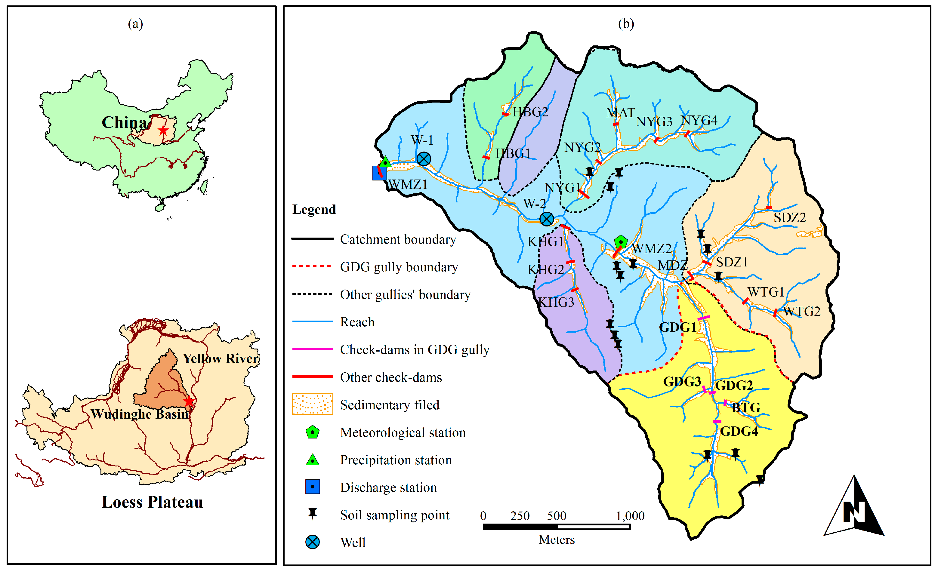
Wangmaogou catchment (WMG) is a loess hilly catchment located near the outlet of Wudinghe Basin, China (Figure 1). The area of the catchment is 5.97 km², and the elevation ranges from 940 to 1188 m a.s.l. Under the impacts of severe soil and water erosion, landscape featured as interlaced gullies are formed gradually, with a gully density of 4.3 km/km². The geological structure of WMG is relatively simple: (1) the uppermost layer is 20~30 m deep homogeneous loess soil; (2) the second layer is 50~100 m deep red soil, most of which emerges in the gully head; (3) the underlying bedrock is Triassic sandy shale. WMG catchment has a typical semiarid continental climate. The annual potential evapotranspiration is around 800 mm, while the mean annual precipitation is 513 mm, more than 70% of which is received during the rainy season from June to September [15].

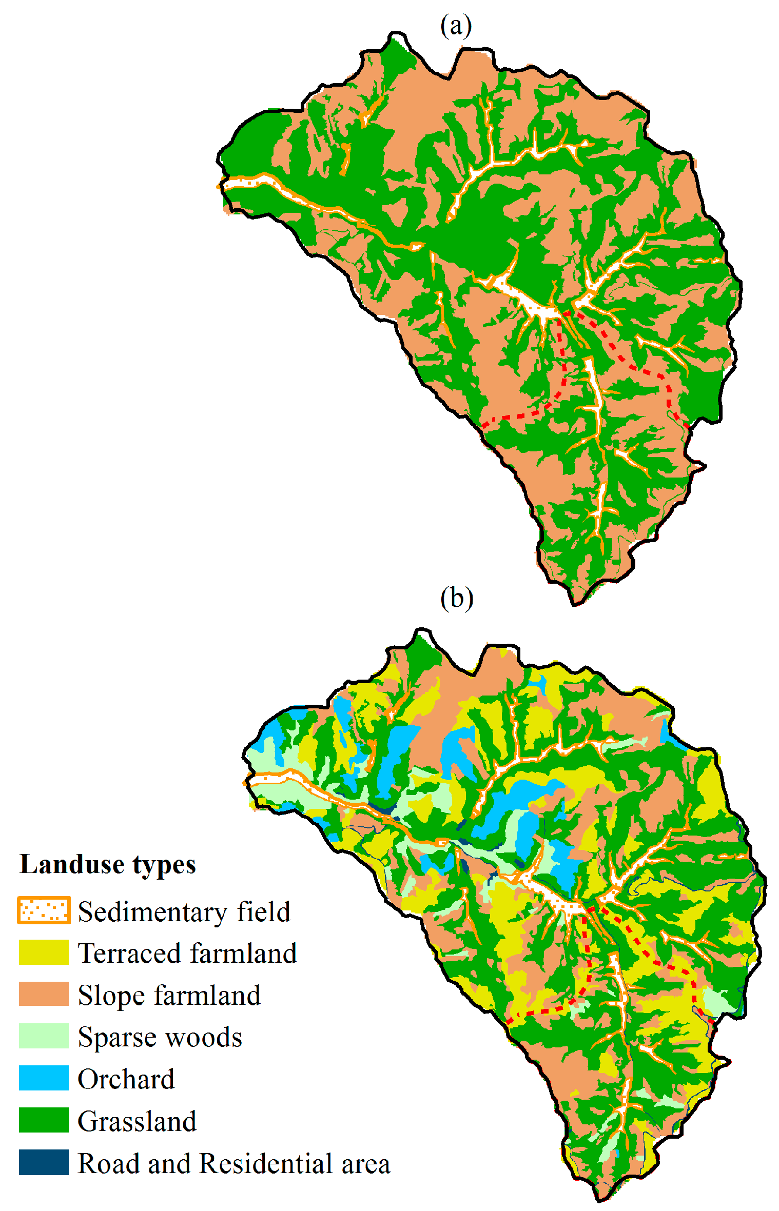
Engineering measures focusing on gully erosion control (i.e., check dams) were carried out in the catchment to alleviate soil and water loss since 1953, before which the average erosion rate was 18,000 t km⁻² per year. 42 check dams were constructed from 1953 to 1959, but most of the dams were destroyed by heavy storms due to low design criteria. Figure 1b shows the 22 currently existing check dams. These check dams have been in operation for more than 50 years under various current conditions (i.e., some have been fully deposited, some have been partially destroyed, the others still remain in good condition). The 42 check dams effectively prevented sediments being transported downstream into Wudinghe River and further into the Yellow River by surface runoff. Other water and soil conservation measures aiming at slope erosion control such as terraced farmlands and woods planting were started in 1962. Figure 2 compares the land use conditions of 1962 and 2010. The primary land use type 50 years ago was slope farmlands (Figure 2a), which was a major erosion source of the catchment. After 50 years, 60% of the slope farmlands were turned into terraced farmlands (Figure 2b), which have a higher water erosion resisting performance. Large areas of grasslands were transformed into sparse woods (Robinta pseudoacacia and Platycladus orientalis) or orchards (apple tree and peach tree) by local farmers.

Table 1. Data set used in this study.

Data Type	Year	Resolution	Data Source	Use in This Study
Land use type	1962, 2010	20-m	Literature [15]	Model construction
Soil data	2014		Field survey	Model construction
Groundwater data	2014	Semi-monthly	Field survey	Model construction
Rainfall-runoff event	10 events during 1962–1964	5-min to 1-hour	Suide Soil and Water Conservation Station	Model calibration
Topography data	1953, 2010	25-m for 1953 map; 5-m for 2010 map	Shaanxi Administration of Surveying [16]	Model construction
Check dam information	1953–1964, 2014		Suide Soil and Water Conservation Station; field survey	Model construction

summarizes the data set used in this study. Detailed field measurements were conducted from April to September 2014. The soil sample tests provide supplemental soil information including saturated hydraulic conductivities (K_sat) and soil water characteristic curves of various land use types at different sampling sites (Figure 1b). Two wells were monitored for water table data set, which was used for calibrating the initial groundwater table. The residual deposition heights (Δh) behind each dam, defined as the height between dam crest and the surface elevation behind the dam, were also carefully measured to present the sedimentary processes. The field data provides a reference for how the catchment functions currently, and serves as validation for the simulated responses. Ten rainfall-runoff events recorded by the local Suide Soil and Water Conservation Station from 1962 to 1964 were used for model calibration. Two topography maps of WMG catchment were used to construct the computational meshes.

Guangdigou catchment (GDG) is a headwater catchment locating in the south of WMG catchment, with a relatively constant dam-system and less land use changes from the 1950s to now. There are five check dams, and

Table 2. Characteristics of the 5 check dams in GDG catchment.

Name	Year 1	Height (m)	Length (m)	Control Area (km2)	Sedimentary Area (× 104 m2)	△h 2 (m)
GDG1	1955 (1959) 3	10 (+13) 3	66	1.14	2.81	7.00
GDG2	1959	8	28	0.10	0.24	1.00
GDG3	1959	12	36	0.05	0.24	1.10
GDG4	1959	8	46	0.40	1.00	2.90
BTG	1959	10	45	0.20	0.94	0.80

¹ Completion year, all dams were completed before the rainy season.; ² △h is the residual deposition height, measured in April 2014.; ³ GDG1 dam was heightened by 13 m in 1959.

shows the characteristics of them.

As shown in Figure 1b, GDG1 is located near the outlet of the main gully and installed in series with GDG2 and GDG4 along the main gully. GDG3 and BTG are located on the outlet of two tributary gullies. The five dams are still in good condition. Compared to other sub-catchments in WMG, the landuse change of GDG was relatively simple during the 50 years, with a large area of slope farmlands being replaced by terraced farmlands.

2.2. The Integrated Hydrology Model (InHM)

Based on the blueprint of the distributed physics-based hydrological model proposed by Freeze and Harlan [17], InHM was developed to quantitatively simulate, via a fully coupled approach, 3-dimensional variably saturated flow in soil and 2-D flow and sediment transport across land surface [18,19,20,21]. The 3-D Richards’ equation was implemented to describe variably saturated flow in soil, while the 2-D diffusion-wave equation coupled with depth-integrated multiple-species sediment transport was applied to describe surface flow movement and sediment transportation. Those surface and subsurface governing equations were discretized in space using the control volume finite element method and coupled in one coherent framework using physics-based first-order flux relationship driven by pressure head gradients. Newton iteration was used to implicitly solve each coupled system of nonlinear equations. More details of InHM can be found in Appendix A.

With the most important and innovative characteristic (i.e., no priori assumption of specific runoff-generation mechanisms), InHM has been successfully employed in many different catchments across the world for event-based or continuous hydrological-response simulations [22,23] as well as hydrologically-driven sediment transport simulations [24,25]. In the Loess Plateau catchments of Wangmaogou and its sub-catchment Guangdigou, InHM is capable of simulating rainfall-runoff processes dominated by the infiltration-excess surface flow mechanism and also rainsplash and hydraulic erosion processes in flood events. Spatially distributed information (e.g., surface flow velocity and sediment flux) of these processes can be provided by the model.

2.3. Scenario Setting and Modelling Procedure

Two simulation stages were designed in this study. The first stage is calibration and validation simulations, to obtain the actual values of important and sensitive parameters. In the second stage, which was the focus of the study, annual continuous simulations were conducted to evaluate the hydrologic effects and sedimentary processes of a check dam system. The effects of check dam operation in the early period (1955–1962) and in the current period (2010–2013) were both studied. In the second stage, the model took us to “revisit” what had happened in the first few years after the construction of check dams and compared the water table changes and sedimentary processes of the current dam-system with the early dam-system.

2.3.1. Calibration and Validation Simulations in WMG Catchment

Calibration and validation simulations were conducted in WMG catchment, using the data of ten rainfall-runoff events recorded at the discharge station (Figure 1b) from 1961 to 1965, which were the only available observation data (Table 1). Four events were used for calibration and the other six events were used for validation. For a specified flood event, check dams were manually added/removed from the mesh according to their status (already existing or destroyed) during the event.

Simulated water discharges and sediment discharges were compared with observed values and the preliminary results were improved by adjusting surface and subsurface parameters of InHM. Parameters, related to infiltration and runoff-generation (i.e., saturated hydraulic conductivity and Manning’s roughness coefficient) and erosion (i.e., rainsplash coefficient and surface erodibility), were carefully adjusted to improve the simulated results in the course of calibration. The Nash and Sutcliffe modelling efficiency (EF) [26], given by Equation (1), was employed here to evaluate the model performance.

$$EF=\left[{\displaystyle \sum _{i=1}^n{(O_i-\overline{O})}^2-{\displaystyle \sum _{i=1}^n{(S_i-O_i)}^2}}\right]/{\displaystyle \sum _{i=1}^n{(O_i-\overline{O})}^2}$$

(1)

where O_i was the observed value (water discharge or sediment discharge), $\overline{O}$ was the average value of the observed values, and S_i was the simulated value and n was the number of samples. Considering the lack of available measurements to provide land surface information of WMG catchment from 1955 to 1962, these calibration and validation efforts helped to obtain important parameters (e.g., calibrated K_sat for various soil types) to construct a more realistic boundary-value problem for the following simulations.

2.3.2. Annual Continuous Simulations in GDG Catchment

Using the calibrated parameters but different meteorological and land use data, annual continuous simulations were carried out for research period 1953–1962 and 2010–2013. It should be noticed that we had to use event-based calibrated parameters to conduct annual continuous simulations because of the lack of long-term observation data. Considering the fact that most of the observed runoff events in a year only occurred in several rainfall storms in the catchment and InHM performed reasonably well in the ten rainfall-runoff events with various rainfall characteristics (rainfall intensity, rainfall amount and duration, see details in Section 3.1), it was technically sound to conduct the following annual continuous simulations using event-based calibrated parameters.

A WMG-catchment boundary-value problem (BVP) was first built to conduct the calibration simulations in the first stage because the discharge station was located at the outlet of WMG catchment. Another BVP was needed to simulate the influence of check dams because: (1) it was difficult to evaluate the hydrologic effects and sedimentary processes of a complicated check dam system which contained 42 check dams 50 years ago and only 22 now; (2) different land use types of WMG catchment after the construction of check dams also increased the degree of complexity. To simplify the problem, the GDG sub-catchment, within WMG with a relatively constant dam-system and less land use changes, was chosen as an example to study the effects of check dams. As mentioned above, the geological structure of WMG was relatively simple. The soil types and features of GDG gully were the same as those of the rest part of WMG catchment. The parameters calibrated in the WMG BVP were mainly related to soil characteristics (e.g., saturated hydraulic conductivity, rainsplash coefficient) and could be directly used in GDG BVP. It was technically reasonable to conduct the GDG BVP simulations using parameters from WMG BVP simulations.

Four scenarios were designed in this study to evaluate the impacts of check dams on hydrologic response and the sedimentary processes (

Table 3. Description of the four scenarios in the study.

Scenario Name	Simulation Time Range	Check Dam Involved
Pre-dam (PD)	1953–1954	none
Single-dam (SD)	1955–1958	GDG1
Early dam-system (EDS)	1959–1962	GDG1–4, BTG
Current dam-system (CDS)	2010–2013	GDG1–4, BTG

). Pre-dam scenario (PD) represented the situation before the construction of the first check dam (i.e., base case), with a two-year simulation because the available precipitation data started in 1953. Single-dam scenario (SD) represented the situation after the construction of GDG1 dam in the downstream. Early dam-system scenario (EDS) represented the conditions after four extra dams (i.e., GDG2-4, BTG) were constructed in the upstream of the gully. Current dam-system scenario (CDS) represented the current conditions including large areas of terraced farmlands and a more than 50-year-old check dam system.

The impacts of check dams on water redistribution were compared among the four scenarios, based on water balance calculation. Changes in groundwater table of channel reach A0-A2 (Figure 3) were analyzed. A series of observation nodes, located on/near the A0-A2 profile at a 5-m (near check dam) and 20 m interval, were set. Pressure head and soil water content were calculated in InHM for each observation nodes at every time step. The surface and subsurface nodes with zero pressure head values together outlined the groundwater table profile of A0-A2 reach. Soil erosion of the GDG catchment in the four scenarios was also evaluated by calculating the eroded sediment mass of different surface zones (

Table 4. Surface parameters used in InHM for the four scenarios.

Scenario	Surface Zone a	Hydrologic Response				Sediment Transport
		n b (-)	ψim c (m)	Ssr d (-)	Ht e (m)	cf f (s m−1)0.6	cd g (1/m)	b h (-)	ξ i (-)	(m−1)
PD	Slope_G	0.10	0.0005	0.01	0.001	4.000	600	1.6	0.25	0.050
	Slope_F	0.12				8.000				0.050
	Gully_G	0.05				4.000				0.050
SD & EDS	Slope_G	0.10				4.000				0.050
	Slope_F	0.12				8.000				0.050
	Gully_G	0.05				4.000				0.050
	Gully_D	0.01				0.001				0.050
	Gully_S	0.05~0.12 k				0.100				0.050
CDS	Slope_G	0.10				4.000				0.038
	Slope_F	0.12				8.000				0.037
	Slope_T	0.50				0.500				0.038
	Gully_G	0.05				4.000				0.040
	Gully_D	0.01				0.001				0.010
	Gully_S	0.05~0.12 k				0.100				0.040

^a The letter behind the underline represents different landuse types: G represents grasslands; F represents slope farmlands; D represents check dams; S represents sedimentary fields caused by dams; T represents terraced farmlands; ^b Manning’s roughness coefficient [20], calibrated from the first stage.; ^c Immobile water depth [20], identical for all surface zones.; ^d Surface residual saturation [20], identical for all surface zones.; ^e Average height of non-discretized micro-topography [20], identical for all surface zones.; ^f Rainsplash coefficient [18], calibrated from the first stage.; ^g Rainsplash depth dampening factor [27], identical for all surface zones.; ^h Rain intensity exponent [27], identical for all surface zones.; ⁱ Rain-induced turbulence coefficient [27], identical for all surface zones.; ^j Surface erodibility coefficient [27], calibrated from the first stage. The values for CDS scenario were derived from Gao et al. [15].; ^k Sedimentary fields are usually used as productive farmlands after averagely 2-year deposition, increasing manning’s roughness coefficient to 0.12.

), which was calculated in InHM by the integration of sediment flux through the boundary we set for each surface zone.

2.4. Model Settings and Parameters

2.4.1. Boundary Conditions and Initial Conditions

The 3D meshes for the four scenarios were all constructed by adding layers to 2D surface meshes. The 2D surface meshes of GDG gully for the first three scenarios were constructed based upon the topographic map surveyed in 1953. A surface mesh with 2165 nodes and 4252 triangular elements was first generated for PD scenario. GDG1 dam was then added to the first surface mesh according to characteristics of GDG1 in Table 2 to generate the second surface mesh for the SD scenario, which has 2243 nodes and 4408 triangular elements. The other four dams were then added on the second mesh to generate the third surface mesh for EDS scenario (Figure 3), which consists of 2499 nodes and 4920 triangular elements. The fourth surface mesh for CDS scenario, which has 2451 nodes and 4799 triangular elements, was generated using the DEM in 2010 with 5 m horizontal resolution. The discretization of all the surface meshes varied from 50 m along the boundary to 20 m along the gullies and 5 m on the five check dams. 30 subsurface layers were added below the surface mesh. Considering that the 0.5 m deep soil near surface is the most sensitive to land use changes and important for surface hydrology, a constant thickness of 0.05 m was assigned to the first ten sublayers. The second ten sublayers (layer 11 to layer 20) had a uniform thickness of 0.5 m. A base elevation of 976.5 m (the elevation of GDG gully ranges from 992 to 1188 m a.s.l) was set as the bottom of the 3D mesh, creating variable thickness for the third ten layers (layer 21 to layer 30).

The vertical discretization for layer 21 to layer 30 ranged from 1.0 m near gully’s outlet to 20.5 m at the boundary upland of the gully. This discretization method both ensured a fine resolution in the hydrologically active areas (i.e., the channel, sedimentary land, and the near-surface soil) and simultaneously saved computation resources in the relatively inactive areas (i.e., the headwater regions and deep spaces).

Using a similar method as Heppner and Loague [24], the initial 3D pressure-head distribution of GDG-gully for PD scenario was generated by conducting a one-year quick-drainage simulation starting from the following condition:

$${\psi }_{t=0}=\{\begin{array}{ll}0.992\times z_{surf}-z,& z_{surf}\le 1060\\ -0.34\times z_{surf}-z+1411.92,& z_{surf}>1060\end{array}$$

(2)

where ${\psi }_{t=0}$[L] was the initial pressure head of the simulation for a certain node, $z_{surf}$[L] referred to the surface elevation directly above the node and $z$[L] was the elevation of the node. 1060 m-contour was the typical dividing line of gully and slope. The choice of the initial condition for the one-year simulation was motivated by the fact that the groundwater table of the north-western Loess Plateau is around 5~10 m below surface in gullies and nearly 50~150 m below surface for slopes. This quick-drainage simulation used a synthetic rainfall time-series which only contained several small rainfall events to represent a dry year before 1953. A self-consistent head distribution, obtained from the quick-drainage simulation, was assigned to the first GDG-gully BVP (i.e., PD scenario). The initial conditions of SD scenario and EDS scenario were gleaned from the simulation results of PD scenario and SD scenario, respectively. The initial pressure head values for newly added nodes in SD scenario and EDS scenario were determined as the weighted average values of the nearest eight nodes.

To generate the initial 3D pressure-head distribution for CDS scenario, another quick-drainage simulation for the whole WMG catchment was conducted starting from the following condition:

$${\psi }_{t=0}=\{\begin{array}{ll}0.999\times z_{surf}-z,& z_{surf}\le 1060\\ -0.34\times z_{surf}-z+1419.34,& z_{surf}>1060\end{array}$$

(3)

The choice of 0.999 in the first part of Equation (3) generated a high water-table shape along gullies at the beginning of the simulation. Then, the quick-drainage simulation started with no flux applied at the surface and ended when the simulated water table depths matched with observed average water table depths at the well-1 and well-2 (i.e., 8.0 m and 5.0 m, respectively) in Figure 1b. The pressure head values of all subsurface nodes for GDG catchment were extracted from the drainage simulation and assigned to the fourth GDG gully-BVP (i.e., CDS scenario) as initial subsurface conditions.

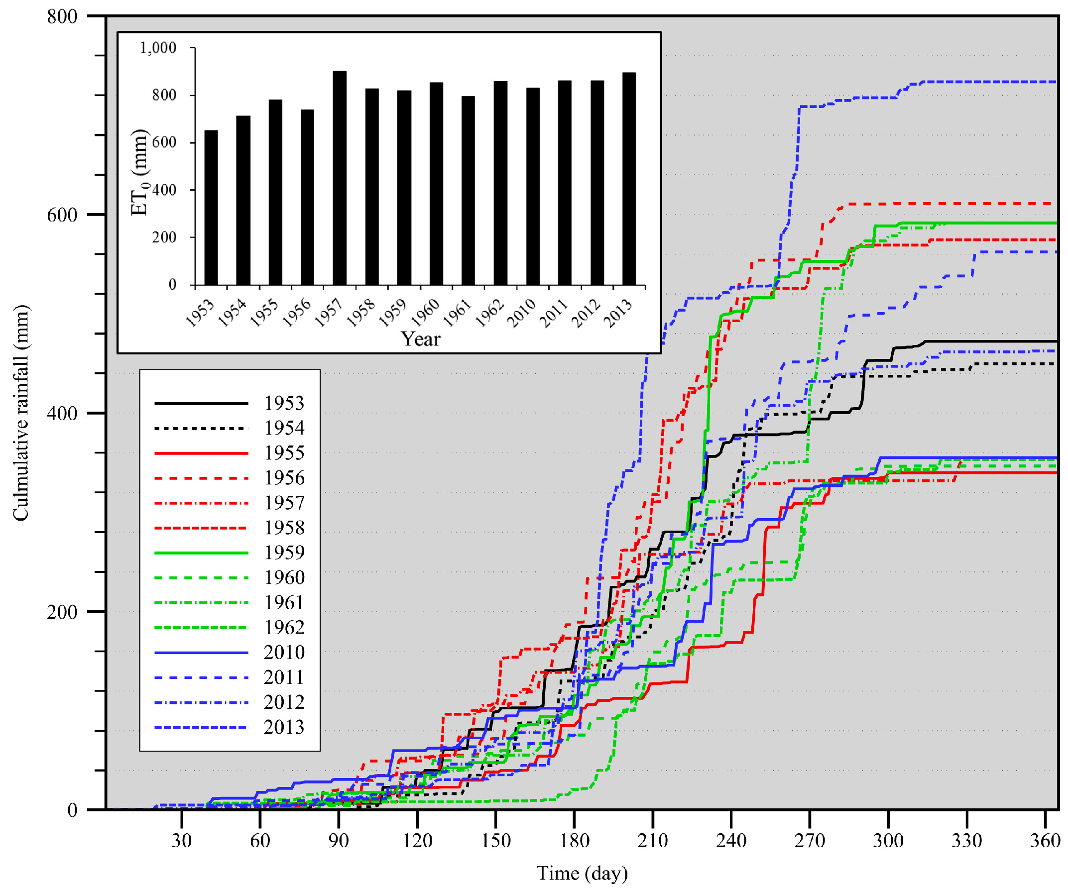
Three subsurface boundary conditions were assigned to the 3D boundary-value problems: (1) impermeable for each lateral face; (2) leaking at the saturated hydraulic conductivity for the basal boundary; (3) a local sink (i.e., head-dependent flux) at the down-gradient face. Specified fluxes for precipitation and evapotranspiration and a critical depth (d = 0 m) at the gully outlet were the three surface boundary conditions. The rainfall time-series spanning from 1953 to 1962 for the former 3 scenarios and from 2010 to 2013 for the CDS scenario were obtained from the precipitation station (Figure 1b). Figure 4 shows the cumulative rainfall and annual potential evapotranspiration (ET₀) for all the simulation years. The FAO56 recommended revised-Penman-Monteith method was used to estimate the daily potential evapotranspiration, using meteorological data such as daily temperature, daily vapor pressure, daily atmospheric pressure, daily solar radiation and wind speed from the meteorological station. The calculated daily potential evapotranspiration was then incorporated into InHM as actual evapotranspiration (ET) using a set of sink functions [22]:

$$Q_b^E=\alpha (\psi )q_{\max }^E{A}_b$$

(4)

where $Q_b^E$[L³T⁻¹] represented the volumetric evapotranspiration rate, $\alpha (\psi )$[–] was a response function of the saturation of the porous medium and the degree of ponding at the land surface, $q_{\max }^E$[LT⁻¹] was the potential evapotranspiration rate per unit area estimated by the revised Penman-Monteith method, $\psi$[L] was the pressure head of the subsurface nodes or water depth of the surface nodes, and $A_b$[L²] was the area associated with the surface water equation.

2.4.2. Soil Parameters

Soils were classified as one layer of surface soil (0~20 cm) and two layers of subsurface soil (20~50 cm and below 50 cm). The surface soil layer was furtherly divided into six types according to land covers. Several soil parameters influencing hydrologic response and sediment transport were determined by field measurements or derived from the literature (Table 4). For example, the saturated hydraulic conductivity (K_sat) values for CDS scenario were measured in April 2014, while K_sat values for the other three scenarios were obtained via model calibration. Derived from the previous studies based on soil texture, the damping coefficient, raindrop turbulence factor, and rainfall intensity exponent were, respectively, set to 600 m⁻¹, 0.25, 1.6 [25,28]. Manning’s roughness coefficient and rainsplash coefficient were obtained from model calibration. Surface erodibility coefficient for the first 3 scenarios was calibrated to 0.050. The surface erodibility coefficients for CDS scenario, lower than calibrated value, were derived from the work by Gao et al. [15] to represent the current surface condition. van Genuchten [29] equation was employed to describe the soil water characteristics and the parameters of the equation (

Table 5. Soil parameters used in InHM for the four scenarios.

Scenario	Subsurface Zone	Ksat (m s−1)	Porosity (-)	Sr a (-)	α b (m−1)	n c (-)
PD	Slope_G d	6.20 × 10−7	0.4800	0.0900	1.29	1.630
	Slope_F d	3.40 × 10−6	0.4500	0.1000	1.27	1.710
	Gully_G d	3.50 × 10−6	0.4800	0.0900	1.40	1.650
	20~50 cm e	5.00 × 10−6	0.4500	0.0976	1.20	1.503
	Below 50 cm e	3.00 × 10−6	0.4000	0.1000	0.92	1.542
SD & EDS	Slope_G d	6.20 × 10−7	0.4800	0.0900	1.29	1.630
	Slope_F d	3.40 × 10−6	0.4500	0.1000	1.27	1.710
	Gully_G d	3.50 × 10−6	0.4800	0.0900	1.40	1.650
	Gully_D e	3.23 × 10−8	0.2500	0.0599	1.01	1.374
	Gully_S e	3.19 × 10−5	0.5000	0.0931	3.05	1.667
	20~50 cm e	5.00 × 10−6	0.4500	0.0976	1.20	1.503
	Below 50 cm e	3.00 × 10−6	0.4000	0.1000	0.92	1.542
CDS	Slope_G e	8.45 × 10−7	0.5068	0.1176	1.74	1.579
	Slope_F e	2.18 × 10−6	0.4268	0.0929	1.50	1.601
	Slope_T e	7.81 × 10−6	0.4819	0.0833	2.19	1.735
	Gully_G e	3.96 × 10−6	0.4640	0.0888	1.63	1.704
	Gully_D e	3.23 × 10−8	0.2500	0.0599	1.01	1.374
	Gully_S e	3.19 × 10−5	0.5221	0.0931	3.05	1.667
	20~50 cm e	5.00 × 10−6	0.4500	0.0976	1.20	1.503
	Below 50 cm e	3.00 × 10−6	0.4000	0.1000	0.92	1.542

^a Residual soil-water content.; ^b Parameter related to the inverse of the air-entry pressure [29].; ^c Parameter related to the pore-size distribution [29].; ^d Values were all calibrated in WMG BVP.; ^e Values were all measured in April 2014.

) for loess soils were derived from infiltration experiments conducted in WMG catchment. According to the soil sample data in the catchment, the median diameter of the soil was set to 0.05 mm to represent the uppermost homogeneous loess soil and a single species particle with a particle density of 2650 kg·m⁻³ was used for all soil layers for the sediment transport simulation. The soil cohesion coefficient was 0.30 [24] for all surface soil except that of the check dam body, which was assigned a larger cohesion coefficient (i.e., 0.60) due to compaction.

3. Results and Discussion

3.1. Results of Calibration and Validation in WMG Catchment

Table 6. Comparisons of observed versus simulated results for 10 rainfall-runoff events in the first simulation stage.

N a	Date	P (mm)	Qpk (m3/s) b		Tpk (h) c		EFh d	Qs, pk(Kg/s) b		Ts, pk(h) c		EFs d
			O	S	O	S		O	S	O	S
1	1962/7/15	29.3	1.90	1.62	5.8	5.4	0.78	1276	890	5.8	5.7	0.71
2	1963/7/05	64.8	0.58	0.48	6.9	7.1	0.79	37	25	6.9	7.3	0.72
3	1964/9/07	26.8	1.60	1.59	11.5	11.6	0.71	133	120	11.5	11.6	0.72
4	1965/7/07	19.0	0.20	0.15	2.5	2.6	0.93	7	8	2.3	2.5	0.88
5	1961/7/05	46.3	1.50	1.32	5.7	6.0	0.59	93	74	5.7	6.0	0.60
6	1961/8/01	54.7	21.00	12.12	2.8	4.0	0.71	9240	4863	2.8	5.0	0.41
7	1961/9/27	35.2	1.53	1.10	4.9	5.3	0.68	137	91	4.9	4.9	0.62
8	1964/7/05	133.1	7.07	4.61	16.1	16.0	0.60	4242	3726	16.1	16.3	0.50
9	1964/7/12	24.6	1.63	1.43	5.2	5.3	0.56	904	681	5.2	5.1	0.69
10	1964/9/11	51.4	1.82	1.63	8.1	8.0	0.65	820	777	8.1	8.0	0.45

^a Event number. Events 1 to 4 were used for calibration, and events 5 to 10 were used for validation.; ^b Q_pk referred to the peak discharge, and Q_s, _pk was the peak sediment discharge.; ^c T_pk referred to the time to Q_pk from the start of the event, and T_s, _pk was the time to Q_s, _pk from the start of the event.; ^d EF_h referred to the EF value for hydrologic-response simulation, and EF_s was the EF value for sediment-transport simu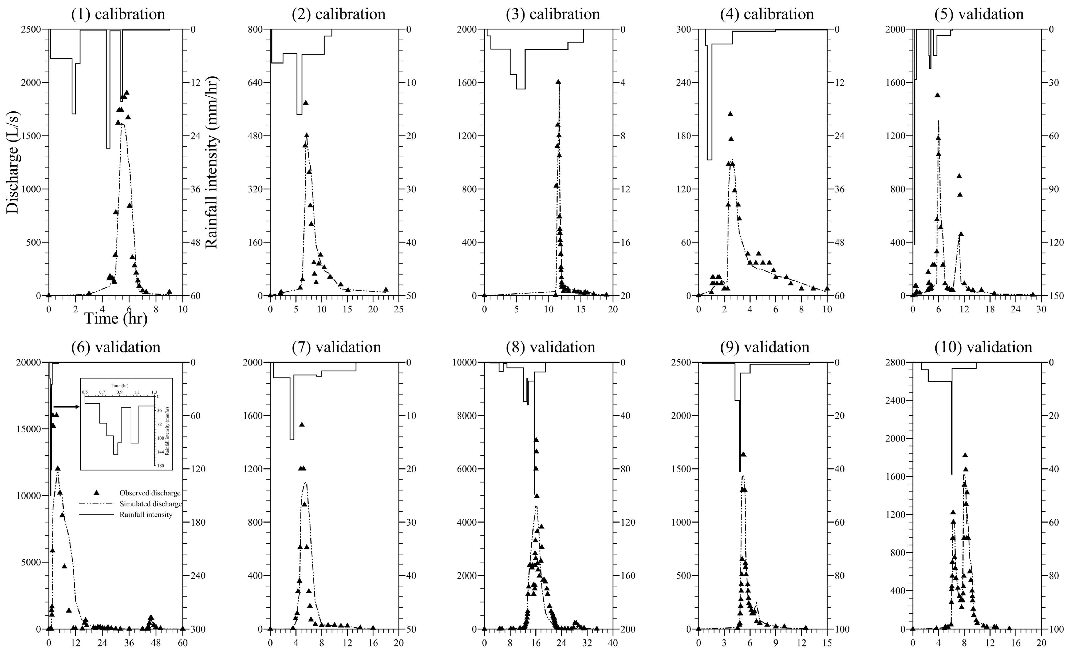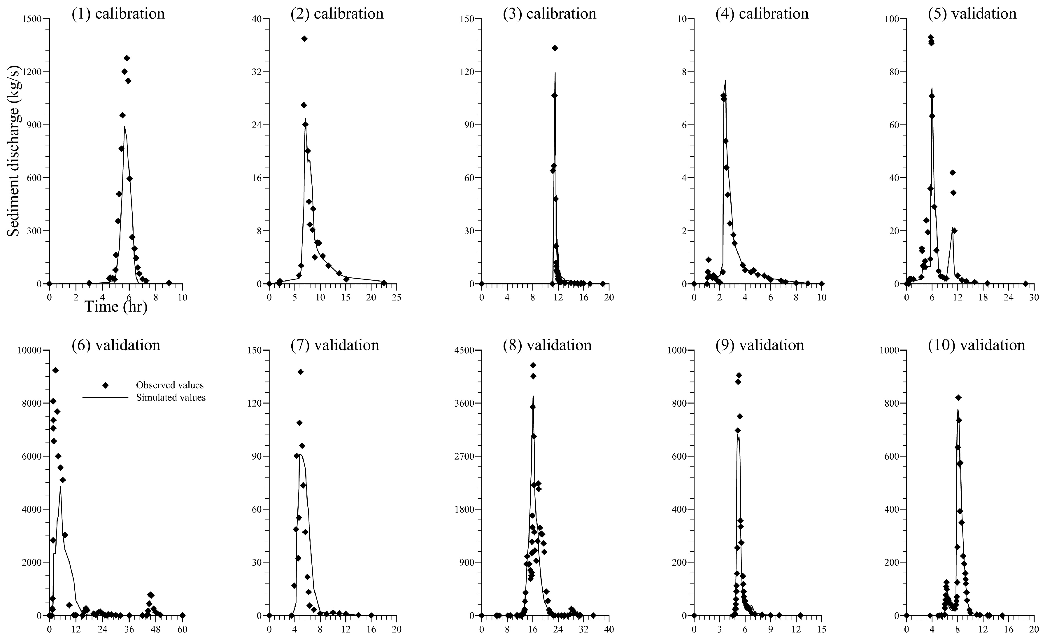lation.

compares the observed and simulated peak discharges and the time to peak discharges of water and sediment of the ten rainfall-runoff events. EF values for water discharge and sediment discharge were calculated, separately. The EF values in the four calibration events were all higher than 0.70, and the model produced the best simulation results in event 4, which was characterized as low rainfall intensity and rainfall amount with low water and sediment discharges. The average EF values of water discharge and sediment discharge for the six validation events were all higher than 0.55, illustrating that model performances were acceptable both in water discharge simulation and sediment discharge simulation. The observed and simulated hydrographs (Figure 5) and sedigraphs (Figure 6) for the 10 events matched reasonably well, also indicating a good representation of the hydrologically-driven sediment transport processes.

3.2. Water Redistribution in Long-Term Simulations of GDG Catchment

Table 7. Water redistribution in long-term simulations of GDG catchment.

Scenario	Year	Precipitation (mm)	Outflow (%)		Storage Change (%)		ET (%)
			Surface	Subsurface	Surface	Subsurface
PD	1953	476.50	15.00	5.00	0.80	1.70	77.50
	1954	449.30	14.32	3.94	1.00	−0.63	81.37
	Average	462.90	14.66	4.47	0.90	0.54	79.43
SD	1955	326.90	1.01	4.51	8.94	4.93	80.61
	1956	610.88	2.11	7.35	3.20	11.01	76.33
	1957	354.70	1.36	7.54	3.18	8.69	79.23
	1958	574.50	3.20	9.27	2.24	15.10	70.19
	Average	466.75	1.92	7.17	4.39	9.93	76.59
EDS	1959	590.80	4.39	8.74	18.37	11.09	57.41
	1960	346.70	1.03	12.31	4.87	14.99	66.80
	1961	591.11	2.57	10.74	8.96	12.38	65.35
	1962	353.00	0.97	14.17	3.01	6.74	75.11
	Average	470.40	2.24	11.49	8.80	11.30	66.17
CDS	2010	355.00	1.12	9.79	1.64	10.24	77.21
	2011	562.30	3.71	11.62	1.02	12.12	71.53
	2012	462.70	3.58	11.69	0.67	9.10	74.96
	2013	733.70	3.08	13.15	2.79	8.88	72.10
	Average	646.03	2.90	11.56	1.53	10.09	73.92

provides the InHM simulated GDG water-balance components for each year of the four scenarios. Precipitation of each year was redistributed into three water-balance components (i.e., outflow, storage change, and evapotranspiration). Surface outflow referred to the surface runoff at the outlet of GDG gully, while subsurface outflow included lateral flow leaving the downstream outlet and vertical drainage. Inspection of Table 7 showed that the percentage of each component in the four scenarios was obviously different:

• Surface runoff decreased significantly after the construction of GDG1 dam (i.e., averagely reduced by 12.74%) and remained a low percentage in the following 12 simulation years.
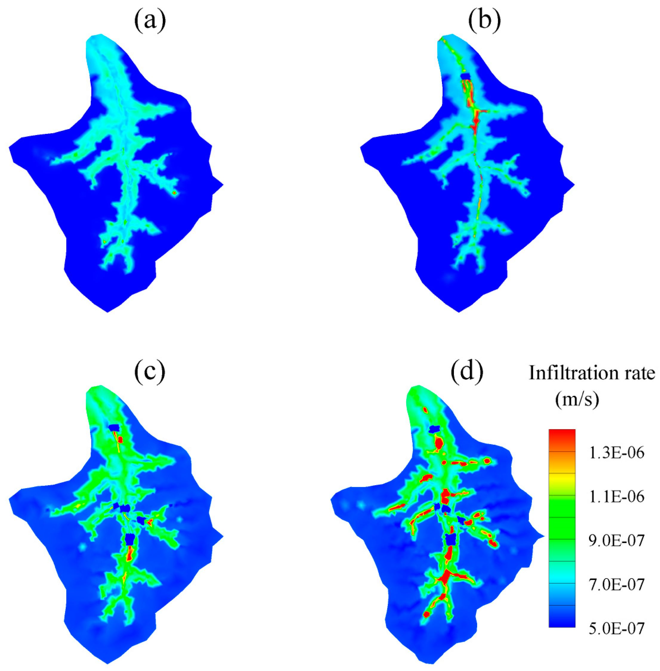
• Surface storage responded in two different ways in the four scenarios. Surface storage dramatically increased by 8.94% and 18.37% immediately at the end of the first year in SD and EDS scenarios, indicating a large amount of stormwater during the rainy seasons of 1955 and 1959 was retained behind check dams. Comparing to the large growth in 1955 and 1959, small increases of surface storage occurred in the following years of SD and EDS scenarios (i.e., 1956, 1957, 1958, 1960, and 1962). PD and CDS scenarios had similarly slight surface storage increases (i.e., average changes were +0.90% and +1.53%, respectively) for different reasons: (1) surface runoff left the gully without the interception of dams in PD scenario; (2) surface water was retained behind dams and infiltrated into subsurface quickly in CDS scenario. (See the expanding permeable sedimentary layers with relatively high infiltration rate in Figure 7)
• Subsurface outflow increased to 7.17% after the construction of GDG1 dam. The mean annual subsurface outflow was 33.5 mm (7.17%) and 54.0 mm (11.49%) for SD and EDS scenarios, increasing by 4.32% after the construction of four more dams. The subsurface outflow remained stable in CDS scenario, fluctuating slightly between wet years and dry years.
• Subsurface storage started increasing significantly in 1956, and fluctuating slightly between dry years and wet years. The check dams’ role in transforming from a surface reservoir to subsurface reservoir was obvious when comparing the storage-change tendencies of the surface and subsurface.
• Evapotranspiration, the largest term in GDG water balance, showed a slight decline from PD to CDS scenarios. It could be explained by the enhancement of infiltration in the sedimentary areas, which reduced the residence time of rainfall as surface water. In SD and EDS scenarios, dry years showed higher ET proportions than wet years.

3.3. Impacts of Check Dams on Groundwater in Long-Term Simulations of GDG Catchment

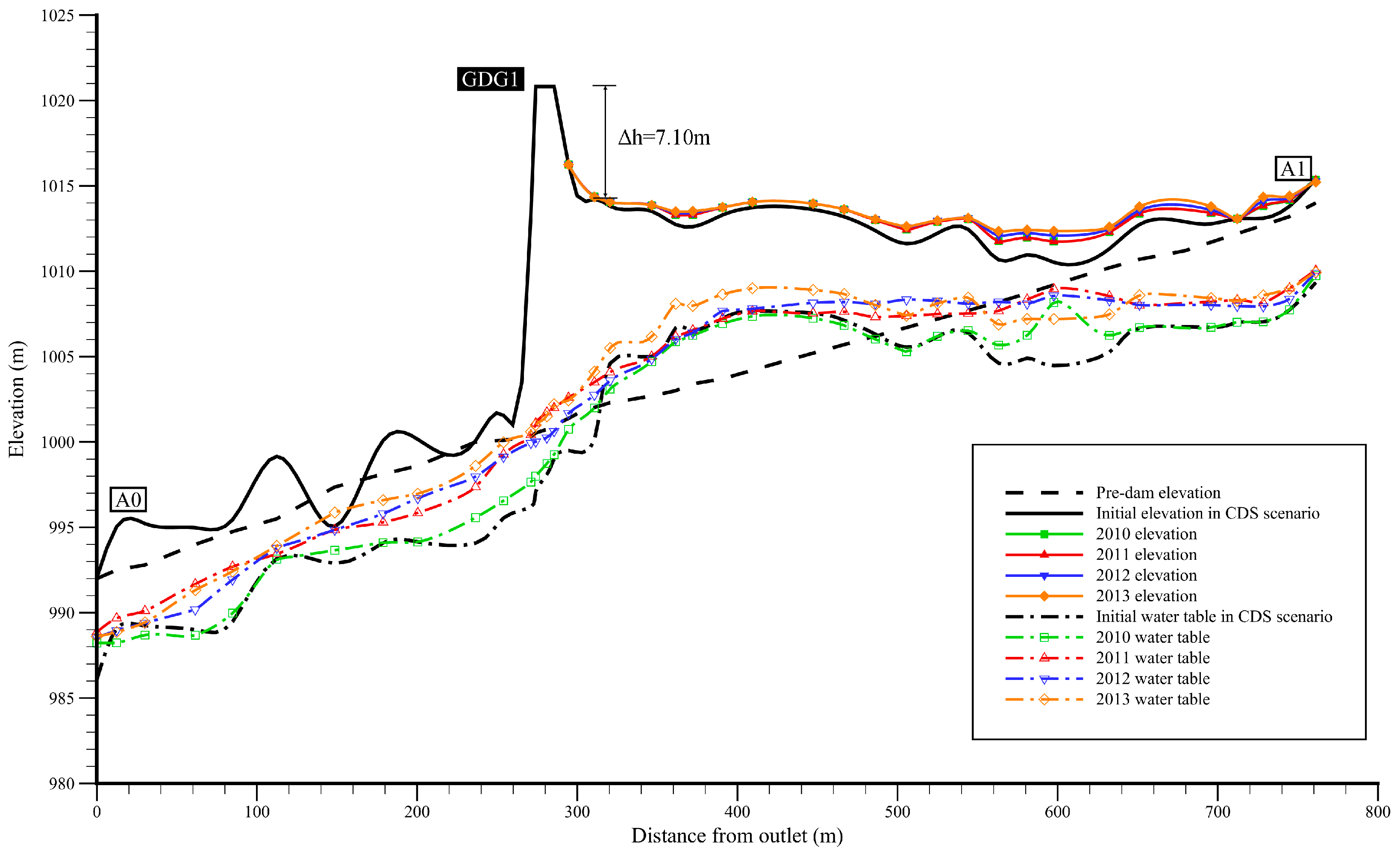
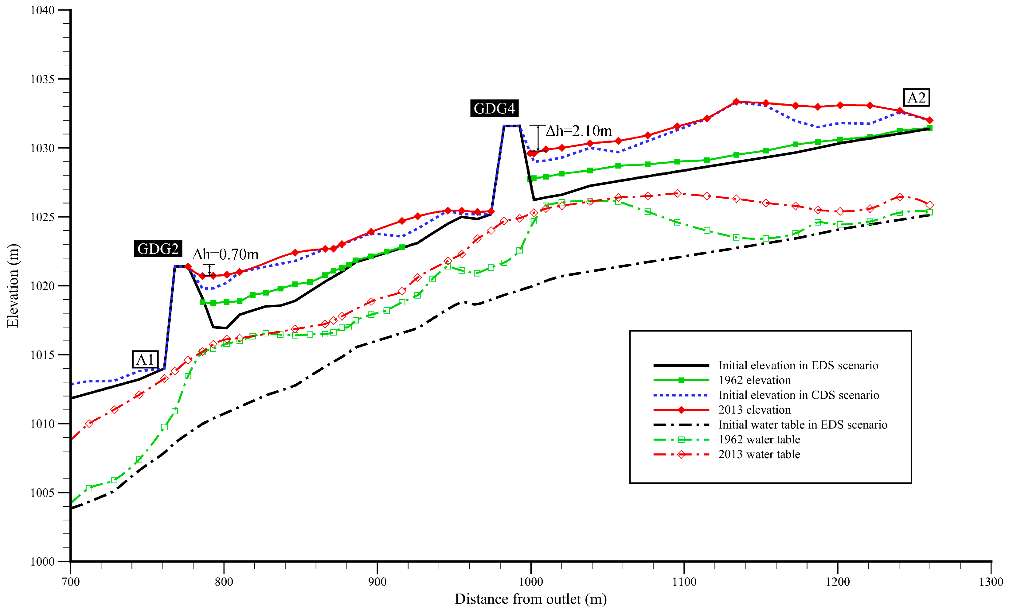
To further capture the influences of check dams on groundwater and the sedimentary processes, the water table profiles and surface elevations along the gully of each year were compared (Figure 8, Figure 9, Figure 10 and Figure 11). The impacts of check dams on the GDG1 dam-controlled reach (i.e., A0-A1 reach in Figure 3) in different stages (i.e., SD, EDS, and CDS) are compared in Figure 8, Figure 9 and Figure 10. Figure 11 compared the water table changes and sedimentary processes of the two-dam reach (i.e., A1-A2 reach in Figure 3) in EDS and CDS scenarios. Perusal of the water table changes lead to the following results:

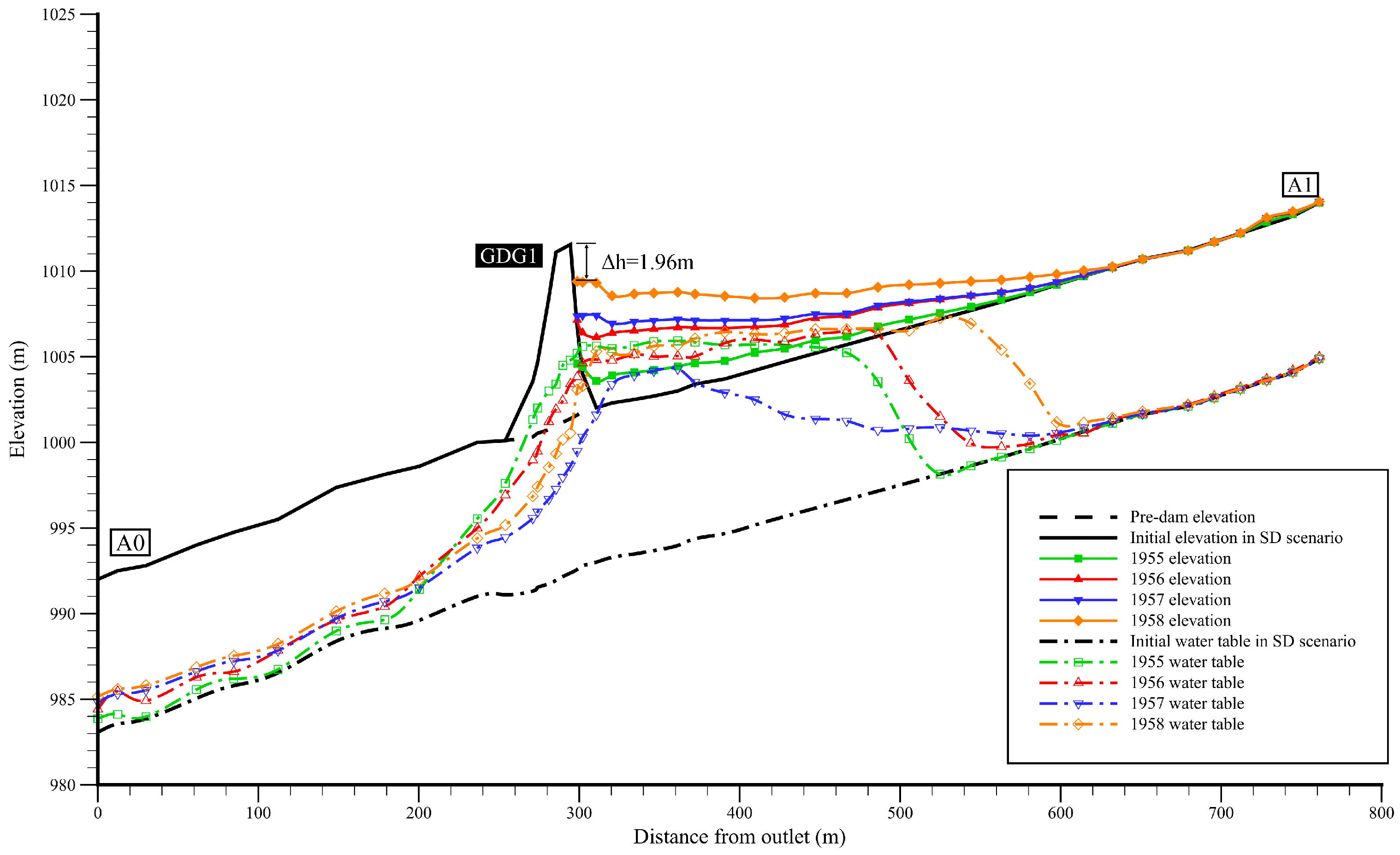
• The water table rose sharply at 200 m upstream from the dam heel of GDG1 and dropped sharply at the dam toe at the end of 1955 (see the green dash line with square symbols in Figure 8), indicating the formation a “subsurface reservoir”.
• Surface ponding was found in the first year of SD scenario (also see the green line in Figure 8) and disappeared in the following years.
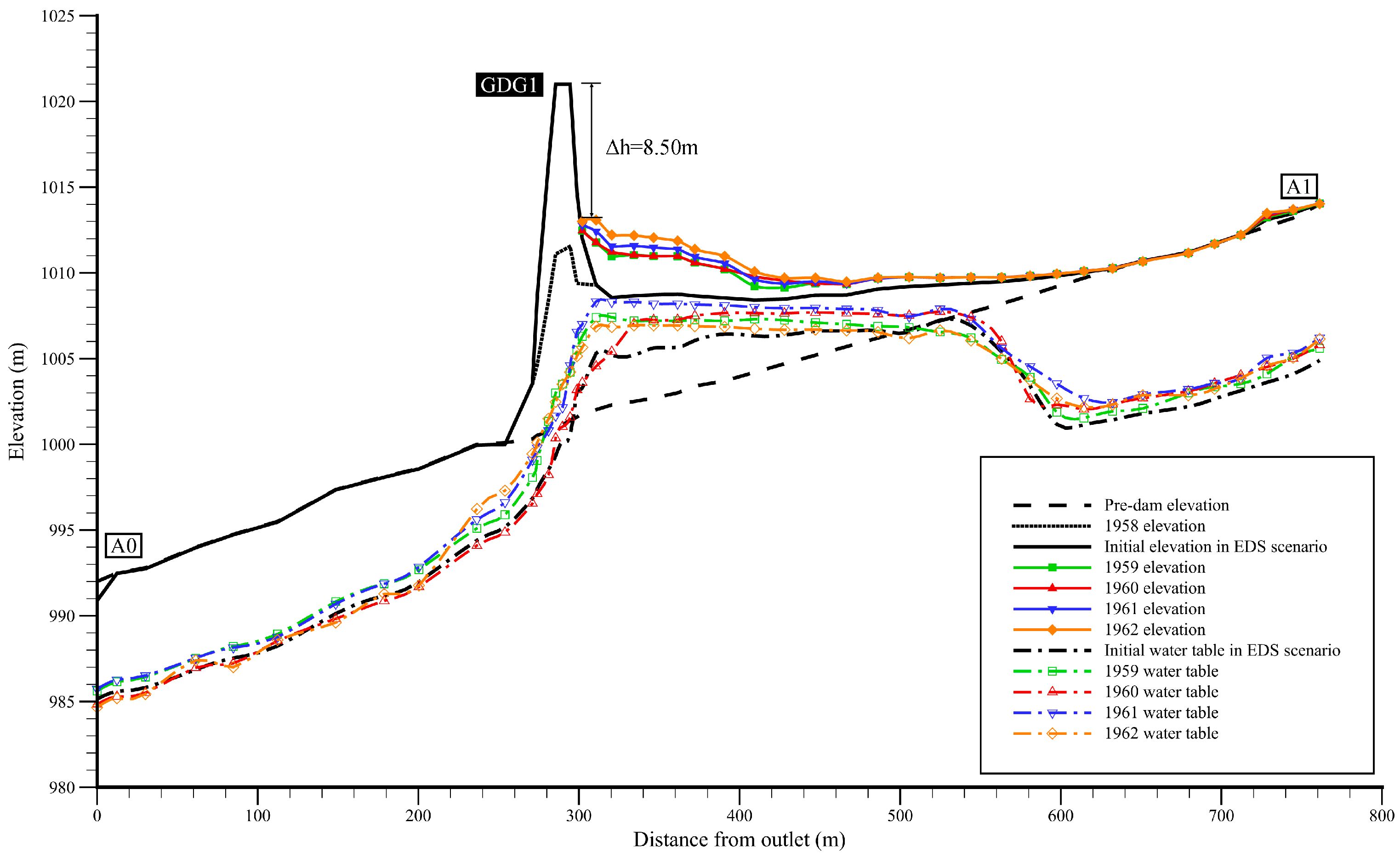
• The position where water table started rising moved upstream to the location 320 m away from the dam heel of GDG1 at the end of 1958 (see the orange dash line with diamond symbols in Figure 8) and remained there in EDS scenario (Figure 9), indicating the expansion of “subsurface reservoir” referred above.
• The water table downstream the dam averagely increased by 2.0 m and 0.6 m from the 1st year to the 4th year in SD and EDS scenarios, respectively. However, the water table in the upstream reach remained stable in the SD scenario but averagely rose by 1.0 m in the EDS scenario (see Figure 8 and Figure 9).
• Another difference in water table profiles between SD scenario and EDS scenario was the sensitivity to climate. Comparing to the SD scenario, the water table behind GDG1 showed less extreme changes between wet years and dry years in the EDS scenario (see Figure 8 and Figure 9).
• The water table profiles in the CDS scenario (Figure 10) were different from those in the former two scenarios. First, the dam’s impact that caused the water table rising sharply disappeared in CDS scenario. Second, the water table along the gully had risen by 3~5 m both in the upstream reach and in the downstream reach. Third, the water table at the dam toe was relatively high and might expose as springs, which was actually observed during the field survey in April 2014.
• The water table in front of GDG2 and GDG4 in EDS scenario showed similar profile to the water table in front of GDG1 in SD scenario (see the green dash lines with square symbols in Figure 8 and Figure 11). However, the intermediate reach of the two dams (i.e., the reach ranging from 880 m to 980 m away from the outlet) experienced a higher water table lifting (3.0 m averagely), indicating a promotion effect of water table rising by two adjacent check dams (Figure 11).

3.4. Impacts of Check Dams on Sediment Transport in Long-Term Simulations of GDG Catchment

Table 8. Eroded sediment mass of the four simulation scenarios.

Scenario	Year	Eroded Mass (× 104 t)	Eroded Mass of Different Zones (× 104 t) (%)
			Slope_G	Slope_F	Slope_T	Gully_G	Gully_S
PD	1953	3.26	0.85 (26)	1.08 (33)	0.00 (0)	1.34 (41)	0.00 (0)
	1954	3.37	0.94 (28)	1.25 (37)	0.00 (0)	1.18 (35)	0.00 (0)
SD	1955	2.13	0.60 (28)	0.75 (35)	0.00 (0)	0.77 (36)	0.02 (1)
	1956	4.75	1.19 (25)	1.95 (41)	0.00 (0)	1.57 (33)	0.05 (1)
	1957	3.01	0.69 (23)	1.17 (39)	0.00 (0)	1.08 (36)	0.06 (2)
	1958	2.93	1.23 (42)	0.88 (30)	0.00 (0)	0.79 (27)	0.03 (1)
EDS	1959	3.27	0.98 (30)	1.21 (37)	0.00 (0)	0.98 (30)	0.10 (3)
	1960	3.36	0.97 (29)	1.34 (40)	0.00 (0)	0.84 (25)	0.20 (6)
	1961	3.12	0.94 (30)	1.12 (36)	0.00 (0)	0.81 (26)	0.25 (8)
	1962	1.97	0.59 (30)	0.81 (41)	0.00 (0)	0.47 (24)	0.10 (5)
CDS	2010	1.18	0.46 (39)	0.28 (24)	0.12 (10)	0.24 (20)	0.08 (7)
	2011	1.37	0.60 (44)	0.29 (21)	0.16 (12)	0.26 (19)	0.05 (4)
	2012	1.42	0.58 (41)	0.23 (16)	0.26 (18)	0.31 (22)	0.04 (3)
	2013	2.93	1.00 (34)	0.67 (23)	0.41 (14)	0.59 (20)	0.26 (9)

summarizes the eroded sediment mass of each year and the proportion of different zones. The mean erosion moduli, calculated by dividing the eroded mass to the area of GDG gully, was 233.95 t·ha⁻¹·a⁻¹, 226.18 t·ha⁻¹·a⁻¹, 206.77 t·ha⁻¹·a⁻¹ and 121.74 t·ha⁻¹·a⁻¹ for the four scenarios, respectively. Table 8 shows that the eroded sediment mass decreased apparently in CDS scenario. The main reason for the decrease was that slope erosion was directly alleviated by terraced farming, which replaced nearly 60% of slope farmlands with terraced farmlands. For example, 1.17 × 10⁴ t sediment (39%) was eroded from slope farmlands in 1957 (SD scenario with 354.70 mm precipitation). Compared to a similar rainfall condition in 2010 (CDS scenario with 355.00 mm precipitation), only 0.40 × 10⁴ t sediment was eroded from the remaining slope farmlands and the terraced farmlands. Another reason was that gully erosion was indirectly alleviated by the existence of check dams, which formed expanding and elevating sedimentary fields in the channel. For example, the total amount of eroded sediment mass from the two gully-zones (Gully_G, Gully_S) decreased from PD scenario to CDS scenario (Table 8).

Table 9. Observed versus simulated residual deposition height (Δh).

Name	1958			1962			2013
	O a (m)	S b (m)	D c (%)	O a (m)	S b (m)	D c (%)	O a (m)	S b (m)	D c (%)
GDG1	0.50	1.96	292.0	7.90	8.50	7.6	7.00	7.10	1.4
GDG2	-	-	-	3.60	3.90	7.7	1.00	0.70	−30.0
GDG3	-	-	-	6.93	6.20	−10.5	1.10	2.10	90.9
GDG4	-	-	-	4.20	5.10	21.4	2.90	2.10	−27.6
BTG	-	-	-	4.70	5.65	20.2	0.80	1.05	31.3

^a O refers to the observed Δh.; ^b S refers to the simulated Δh.; ^c D refers to Difference = [(Simulated-Observed)/Observed] × 100.

compares the simulated and measured residual deposition heights (Δh) in different stages. Inspection of the surface elevation changes in Figure 8, Figure 9, Figure 10 and Figure 11 and Table 9 helped to revisit the sedimentary processes of GDG gully:

• Deposition in front of GDG1 occurred quickly in SD scenario (1955–1958). The 10 m high check dam was nearly fully deposited and facing the risk of dam-break at the end of 1958 (Figure 8).
• Being heightened by 13 m before the rainy season of 1959, GDG1 was prevented from being over-deposited during the rainy season of 1959 (Figure 9). Less sediment silted in front of GDG1 in EDS scenario due to the existence of the four newly-built dams.
• GDG2 and GDG4, both of which were 8 m high, experienced quick deposition in EDS scenario (see the green solid line with square symbols in Figure 11). GDG3 and BTG, both of which located on the outlet of tributary gullies, also intercepted large amounts of sediment in EDS scenario (Table 9).
• Comparing to PD scenario, a sedimentary layer which has an average thickness of 8 m formed in front of GDG1 dam at the beginning of CDS scenario (see the black solid line in Figure 10). The flat sedimentary area with relatively high soil water content was turned into productive croplands. Long-term alternative erosion and sedimentary formed the undulating terrain in the downstream reach of GDG1. More sediment deposited in the upper reach 600 m away from the outlet rather than at the dam heel for GDG1.
• GDG1, which formed productive croplands, had a residual deposition height (Δh) of 7.10 m at the end of CDS scenario. However, the other four check dams all had been almost fully-filled and were vulnerable to floods.
• Table 9 also shows that most of the simulated Δh values were higher than the observed values (except for GDG3 in 1962, GDG2 and GDG4 in 2013), indicating that the sediment volumes deposited in front of dams were underestimated in most simulations.

3.5. Model Performance Evaluation: Influence of Gravity Erosion

Figure 5 and Figure 6 and Table 6 show underestimations of peak sediment discharges, which were most obvious in event 6 with long-duration high rainfall intensities (i.e., 120–150 mm/h). Most of the simulated residual deposition heights (△h) were larger than the observed ones (8 out of 11), indicating an underestimation of deposited sediment behind check dams (Table 9). For example, the simulated Δh (2.10 m) was nearly two times the observed one (1.10 m) for GDG3 dam in 2013. The most likely reason is that serious collapses occurred on the hillslopes near the two dams. Soils used for constructing check dams were obtained from nearby hillslopes on the two sides of check dams, making the slopes steeper and easier to induce collapse or landslide. According to the inquiries from local farmers, there were several collapses in WMG catchment during the large floods in 27 June 2013 (sediment yield 16,318 tons), one of which occurred on the hillslope near GDG3 dam. Another reason might be the construction of the road on the dam crest. Extra soil from dam crest was poured into the sedimentary area during road construction.

Except for hydraulic erosion, gravity erosion, which usually occurred in the form of landslide or collapse, could dramatically increase sediment yields in a single storm. Since the sediment transport component of InHM was first developed to apply in the hydraulic-erosion-dominating catchments, the sediment transport processes induced by landslides or collapses are not supported yet. Inspiringly, several studies have recently shown the potential of physics-based simulations to forecast landslides and collapses from hydrogeological perspectives (i.e., subsurface fluid-pressures changes in failure-prone locations) [30,31,32]. Future works will be focused on combining the two erosion processes, both of which are related to hydrologic responses, to more accurately predict sediment yields and estimate the sedimentary processes in the Loess Plateau.

4. Conclusions

A comprehensive physics-based model InHM, after model calibration and validation, was employed in a small gully catchment with a more than 50-year-old check dam system. The simulated residual deposition heights reasonably match with the observed values, indicating the ability of InHM in check dam planning and management. The impacts of check dams on the hydrological response and landforms were investigated and the results are summarized as follows.

(1)

Check dams do change the water redistribution in catchment-scale. GDG1 check dam near the gully outlet can effectively reduce surface outflow and increase subsurface outflow. The four other check dams located in the upstream can protect GDG1 from floods risk and promote the redistribution of water.

(2)

The construction of check dam can significantly change the water table profile along the gully. A surface reservoir behind the dam will be formed in the first few years and gradually transformed into a subsurface reservoir, resulting in relatively high soil water content in the sedimentary areas. After more than 50 years of operation, the water table along the gully has been averagely elevated by 3–5 m. Adjacent check dams have a promoting effect on water table rising.

(3)

Check dams intercept surface water and force sediment in the water to deposit. Gully erosion can be alleviated indirectly due to the formation of expanding sedimentary areas.

The simulations reported herein demonstrate that physics-based simulation can provide a framework for better understanding the impacts (both on hydrological response and landform evolution) of check dams in the Loess Plateau. The study is like a “revisit” to the hydrologic and geomorphic changes that occurred after the construction of these dams, and a prediction of what will happen after long-term operation of the dam system, which could be a useful reference in guiding future check dam construction and management. However, as with previous InHM simulations studying the impacts of human activities on the environment, this study also suffered from the difficulty of validation because of lacking observation data that are not only accurate and credible, but also of the correct kind for distributed simulations [22,24]. Although the residual deposition height (Δh) can be used as a reference to prove the simulated sedimentary processes, more detailed measurements on catchment-scale erosion/deposition are needed to aid future physics-based distributed simulations of hydrologic-response-driven geomorphic evolution processes. Furthermore, gravity erosion should be considered in future InHM simulations and more integrated long-term continuous observations such as the groundwater table distribution along the gully and subsurface outflow rates are needed to further guide the search for a comprehensive understanding of hydrologic responses.

References

- Shi, H.; Shao, M. Soil and water loss from the Loess Plateau in China. J. Arid Environ. 2000, 45, 9–20. [Google Scholar] [CrossRef]
- Xin, Z.; Xu, J.; Zheng, W. Spatiotemporal variations of vegetation cover on the Chinese Loess Plateau (1981–2006): Impacts of climate changes and human activities. Sci. China Ser. D Earth Sci. 2008, 51, 67–78. [Google Scholar] [CrossRef]
- Xu, X.; Zhang, H.; Zhang, O. Development of check dam systems in gullies on the Loess Plateau, China. Environ. Sci. Policy 2004, 7, 79–86. [Google Scholar]
- Jin, Z.; Cui, B.; Song, Y.; Shi, W.; Wang, K.; Wang, Y.; Liang, J. How Many Check Dams Do We Need To Build on the Loess Plateau? Environ. Sci. Technol. 2012, 46, 8527–8528. [Google Scholar] [CrossRef] [PubMed]
- Wang, Y.F.; Fu, B.J.; Chen, L.D.; Lu, Y.H.; Gao, Y. Check Dam in the Loess Plateau of China: Engineering for Environmental Services and Food Security. Environ. Sci. Technol. 2011, 45, 10298–10299. [Google Scholar] [CrossRef] [PubMed]
- Xu, Y.; Fu, B.; He, C. Assessing the hydrological effect of the check dams in the Loess Plateau, China, by model simulations. Hydrol. Earth Syst. Sci. 2013, 17, 2185–2193. [Google Scholar] [CrossRef] [Green Version]
- Shi, H.; Li, T.; Wang, K.; Zhang, A.; Wang, G.; Fu, X. Physically-based simulation of the streamflow decrease caused by sediment-trapping dams in the middle Yellow River. Hydrol. Process. 2015, 30, 783–794. [Google Scholar] [CrossRef]
- Boix-Fayos, C.; de Vente, J.; Martínez-Mena, M.; Barberá, G.G.; Castillo, V. The impact of land use change and check dams on catchment sediment yield. Hydrol. Process. 2008, 22, 4922–4935. [Google Scholar] [CrossRef]
- Ran, D.-C.; Luo, Q.-H.; Zhou, Z.-H.; Wang, G.-Q.; Zhang, X.-H. Sediment retention by check dams in the Hekouzhen-Longmen Section of the Yellow River. Int. J. Sediment Res. 2008, 23, 159–166. [Google Scholar] [CrossRef]
- Shi, H.; Wang, G. Impacts of climate change and hydraulic structures on runoff and sediment discharge in the middle Yellow River. Hydrol. Process. 2015, 29, 3236–3246. [Google Scholar] [CrossRef] [Green Version]
- Zhao, P.; Shao, M.; Wang, T. Spatial distributions of soil surface-layer saturated hydraulic conductivity and controlling factors on dam farmlands. Water Resour. Manag. 2010, 24, 2247–2266. [Google Scholar] [CrossRef]
- Callow, J.N.; Smettem, K.R.J. The effect of farm dams and constructed banks on hydrologic connectivity and runoff estimation in agricultural landscapes. Environ. Model. Softw. 2009, 24, 959–968. [Google Scholar] [CrossRef]
- Parimalarenganayaki, S.; Elango, L. Assessment of effect of recharge from a check dam as a method of Managed Aquifer Recharge by hydrogeological investigations. Environ. Earth. Sci. 2015, 73, 5349–5361. [Google Scholar] [CrossRef]
- Huang, J.; Hinokidani, O.; Yasuda, H.; Ojha, C.P.; Kajikawa, Y.; Li, S. Effects of the check dam system on water redistribution in the Chinese Loess Plateau. J. Hydrol. Eng. 2013, 18, 929–940. [Google Scholar] [CrossRef]
- Gao, H. Hydro-Ecological Impact of the Gully Erosion Control Works in Loess Hilly-Gully Region. Ph.D. Thesis, The University of Chinese Academy of Sciences, Beijing, China, 2013. [Google Scholar]
- Shaanxi Administration of Surveying, Mapping and Geoinformation. Available online: http://www.shasm.gov.cn/ (accessed on 4 April 2014).
- Freeze, R.A.; Harlan, R.L. Blueprint for a physically-based, digitally-simulated hydrologic response model. J. Hydrol. 1969, 9, 237–258. [Google Scholar] [CrossRef]
- Heppner, C.S.; Ran, Q.; VanderKwaak, J.E.; Loague, K. Adding sediment transport to the integrated hydrology model (InHM): Development and testing. Adv. Water Resour. 2006, 29, 930–943. [Google Scholar] [CrossRef]
- Ran, Q.; Heppner, C.S.; VanderKwaak, J.E.; Loague, K. Further testing of the integrated hydrology model (InHM): Multiple-species sediment transport. Hydrol. Process. 2007, 21, 1522–1531. [Google Scholar] [CrossRef]
- VanderKwaak, J.E. Numerical Simulation of Flow and Chemical Transport in Integrated Surface-Subsurface Hydrologic Systems. Ph.D. Thesis, University of Waterloo, Waterloo, ON, Canada, 1999. [Google Scholar]
- VanderKwaak, J.E.; Loague, K. Hydrologic-response simulations for the R-5 catchment with a comprehensive physics-based model. Water Resour. Res. 2001, 37, 999–1013. [Google Scholar] [CrossRef]
- Carr, A.E.; Loague, K.; VanderKwaak, J.E. Hydrologic-response simulations for the North Fork of Caspar Creek: Second-growth, clear-cut, new-growth, and cumulative watershed effect scenarios. Hydrol. Process. 2014, 28, 1476–1494. [Google Scholar] [CrossRef]
- Mirus, B.B.; Ebel, B.A.; Loague, K.; Wemple, B.C. Simulated effect of a forest road on near-surface hydrologic response: Redux. Earth Surf. Process. Landf. 2007, 32, 126–142. [Google Scholar] [CrossRef]
- Heppner, C.S.; Loague, K. A dam problem: Simulated upstream impacts for a Searsville-like watershed. Ecohydrology 2008, 1, 408–424. [Google Scholar] [CrossRef]
- Ran, Q.; Loague, K.; VanderKwaak, J.E. Hydrologic-response-driven sediment transport at a regional scale, process-based simulation. Hydrol. Process. 2012, 26, 159–167. [Google Scholar] [CrossRef]
- Nash, J.E.; Sutcliffe, J.V. River flow forecasting through conceptual models part 1-a discussion of principles. J. Hydrol. 1970, 10, 282–290. [Google Scholar] [CrossRef]
- Ran, Q. Regional Scale Landscape Evolution: Physics-Based Simulation of Hydrologically-Driven Surface Erosion. Ph.D. Thesis, Stanford University, Stanford, CA, USA, 2006. [Google Scholar]
- Gabet, E.J.; Dunne, T. Sediment detachment by rain power. Water Resour. Res. 2003, 39, 1002. [Google Scholar] [CrossRef]
- Van Genuchten, M.T. A closed-form equation for predicting the hydraulic conductivity of unsaturated soils. Soil Sci. Soc. Am. Proc. 1980, 44, 892–898. [Google Scholar] [CrossRef]
- Mirus, B.B.; Ebel, B.A.; Heppner, C.S.; Loague, K. Assessing the detail needed to capture rainfall-runoff dynamics with physics-based hydrologic response simulation. Water Resour. Res. 2011, 47, W00H10. [Google Scholar] [CrossRef]
- BeVille, S.H.; Mirus, B.B.; Ebel, B.A.; Mader, G.G.; Loague, K. Using simulated hydrologic response to revisit the 1973 Lerida Court landslide. Environ. Earth Sci. 2010, 61, 1249–1257. [Google Scholar] [CrossRef]
- Thomas, M.A.; Loague, K. Hydrogeologic insights for a Devil’s Slide-like system. Water Resour. Res. 2014, 50, 6628–6645. [Google Scholar] [CrossRef]
Figure 1.
(a) Location of WMG catchment (the red star); (b) check dam distributions and measurement locations of soil characteristics and hydrologic data. Polygons with different colors represent different gullies and the red dash line depicts the boundary of GDG catchment.
Figure 2.
Landuse types of WMG catchment: (a) 1962; (b) 2010. The red dash line presents the boundary of GDG catchment.
Figure 3.
3D mesh for EDS scenario, the inset is a downstream view from position A2.
Figure 4.
Measured cumulative rainfall for the 14 simulating years. The inset is the annual potential evapotranspiration (ET0) calculated by the revised Penman-Monteith method.
Figure 5.
Observed and simulated hydrographs for the ten events in the first simulation stage. (1)–(4) were events for calibration, (6)–(10) were events for validation.
Figure 6.
Observed and simulated sedigraphs for the ten events in the first simulation stage. (1)–(4) were events for calibration, (6)–(10) were events for validation.
Figure 7.
Snapshots of infiltration rate at the time of peak discharge of four events with similar rainfall characteristics extracted from the four scenarios, respectively. (a) PD scenario; (b) SD scenario; (c) EDS scenario; (d) CDS scenario.
Figure 8.
Surface elevation changes and water table changes of GDG1 dam-controlled reach during SD scenario. Note that the simulation results in the end of month 11 of each year were used for comparison.
Figure 9.
Surface elevation changes and water table changes of GDG1 dam-controlled reach during EDS scenario. Note that the simulation results in the end of month 11 of each year were used for comparison.
Figure 10.
Surface elevation changes and water table changes of GDG1 dam-controlled reach during CDS scenario. Note that the simulation results in the end of month 11 of each year were used for comparison.
Figure 11.
Surface elevation changes and water table changes of GDG2-GDG4 dam-controlled reach in EDS scenario and CDS scenario. Note that the simulation results in the end of month 11 of each year were used for comparison.