Using Random Forest Classification and Nationally Available Geospatial Data to Screen for Wetlands over Large Geographic Regions

Abstract

Wetland impact assessments are an integral part of infrastructure projects aimed at protecting the important services wetlands provide for water resources and ecosystems. However, wetland surveys with the level of accuracy required by federal regulators can be time-consuming and costly. Streamlining this process by using already available geospatial data and classification algorithms to target more detailed wetland mapping efforts may support environmental planning efforts. The objective of this study was to create and test a methodology that could be applied nationally, leveraging existing data to quickly and inexpensively screen for potential wetlands over large geographic regions. An automated workflow implementing the methodology for a case study region in the coastal plain of Virginia is presented. When compared to verified wetlands mapped by experts, the methodology resulted in a much lower false negative rate of 22.6% compared to the National Wetland Inventory (NWI) false negative rate of 69.3%. However, because the methodology was designed as a screening approach, it did result in a slight decrease in overall classification accuracy compared to the NWI from 80.5% to 76.1%. Given the considerable decrease in wetland omission while maintaining comparable overall accuracy, the methodology shows potential as a wetland screening tool for targeting more detailed and costly wetland mapping efforts.

1. Introduction

Wetlands are a vital natural resource providing habitat for a variety of wildlife and plants, flood and storm surge protection, water quality improvement through treatment of runoff, and recharge of aquifers [1]. However, a significant number of wetlands in the U.S. have been destroyed or repurposed for agricultural or development purposes [2]. The need to protect wetlands is widely recognized and required by federal law and regulations, specifically through Section 404 of the Clean Water Act [3]. Section 404 of the Clean Water Act sets forth a goal of maintaining the nation’s remaining wetland base by avoiding adverse impacts to these ecosystems. To comply with regulations, entities including state departments of transportation (DOTs) must consider potential impacts to wetlands in their infrastructure development projects. DOTs in particular, as well as other organizations, must sufficiently prove that a selected construction plan is the Least Environmentally Damaging Practical Alternative (LEDPA) by, among other tasks, providing wetland delineations [4]. The U.S. Army Corps of Engineers (USACE) evaluates these corridors as the governing authority in wetland permitting.

Although there are a variety of wetland types, all wetlands share common environmental characteristics based on the interaction of hydrology, vegetation, and soil [5]. USACE guidelines for wetland delineation use these common features; they are based on the presence of hydrologic conditions that inundate the area, vegetation adapted for life in saturated soil conditions, and hydric soils [6]. Field verification is the most accurate method to confirm these diagnostic environmental characteristics; however, performing detailed field delineations for large regions can be costly in terms of resources and time. The creation of a screening tool that leverages nationally available georeferenced datasets and modern classification algorithms could aid in the impact assessment process by allowing agencies to target field mapping efforts to smaller areas within a larger region identified as potential wetland areas through the screening process.

The U.S. Fish and Wildlife Service (USFWS) National Wetland Inventory (NWI) is the best example of a national scale inventory of wetland locations in the United States. Initiated in 1974, the NWI is one of the earliest and most commonly used sources of wetland data in the U.S. [7]. NWI maps were intended to provide biologists and others with information on the distribution and type of wetlands to aid in conservation efforts [8]. However, these data were never intended to map federally regulated wetlands [6,9], and research has shown that relying solely on the NWI may fail to protect a significant fraction of wetlands in the U.S. [10]. Limitations of the NWI can be attributed to reliance on manual photointerpretation, which is subjective and may fail to identify certain types of wetlands [11]. Furthermore, the NWI is not funded at a level that would be necessary to conform to the federal wetland mapping standard [8,12].

Coupling nationally available geospatial data with machine learning can offer the opportunity to identify areas within larger regions that have a high likelihood of including wetlands in an automated and repeatable way. Remote sensing is recognized as one of the most useful information sources for wetland identification by the USACE [6], and it has been widely used for wetland studies in the past 50 years [13]. The most commonly used wetland remote sensing data are Landsat multispectral imagery, which as of Landsat 8 is 30 m in resolution for most bands, repeats its cycle every 16 days, includes 11 bands, and is freely available [13]. Researchers have achieved accurate wetland identification results by incorporating Landsat imagery, specifically from the Landsat 8 Operational Land Imagery (OLI) satellite (e.g., [14,15,16,17,18]). At this spatial resolution, however, it is unlikely that approaches could identify exact wetland locations obtained through field delineations by experts, but it is possible that such data could rule out large areas as not being likely to include wetlands.

Machine learning techniques commonly applied in wetland studies include traditional techniques such as Maximum Likelihood classification (e.g., [14,19]) and newer techniques such as random forest classification. Random forest is an ensemble classifier that produces many classification and regression-like trees. Each tree is generated from different bootstrapped samples of training data, and input variables are randomly selected for generating trees [20]. Random forest has become a widely used method for its ability to handle high dimensional data, incorporate both continuous and categorical data, and produce descriptive variable importance measures (e.g., [21,22]). Researchers have used random forest to integrate multispectral imagery, topography, and other ancillary geospatial data for wetland identification (e.g., [12,23,24,25,26]). Furthermore, studies show that random forest can produce higher classification accuracies than traditional techniques for land cover classification (e.g., [17,21,27,28,29]).

While past studies have demonstrated the potential for remote sensing and machine learning frameworks to identify wetlands, they share common elements that limit implementation of their proposed algorithms as a national-scale tool to support environmental planning efforts like those needed by DOTs in the LEDPA process. These limitations include (i) failure to automate workflows making the classification task time-consuming and difficult to replicate, (ii) failure to leverage freely available geospatial data outside of just remote sensing imagery, (iii) inclusion of costly remote sensing data not always available to support environmental planning, and (iv) reliance on software not typically available or used by state DOTs. The objective of this study was to design a methodology that addresses these shortcomings and to implement the methodology as a wetland screening tool in a widely used commercial geographic information system (GIS). As a wetland screening tool, the methodology emphasizes minimizing false negative predictions (i.e., cases of wetland omission) while also maintaining a reasonable overall wetland accuracy. We obtained verified wetland delineations created by experts for a large region (33 km²) in the coastal plain of Virginia to evaluate the methodology. We trained a classification model on a subset of the verified wetland delineation dataset and then tested the classification model using a separate subset of the verified wetland delineation dataset to evaluate its accuracy. Finally, we compared the performance of the wetland tool against the NWI given that this is the standard wetland inventory available for supporting early environmental planning efforts in the absence of more detailed, costly, and time-consuming field surveys.

2. Materials and Methods

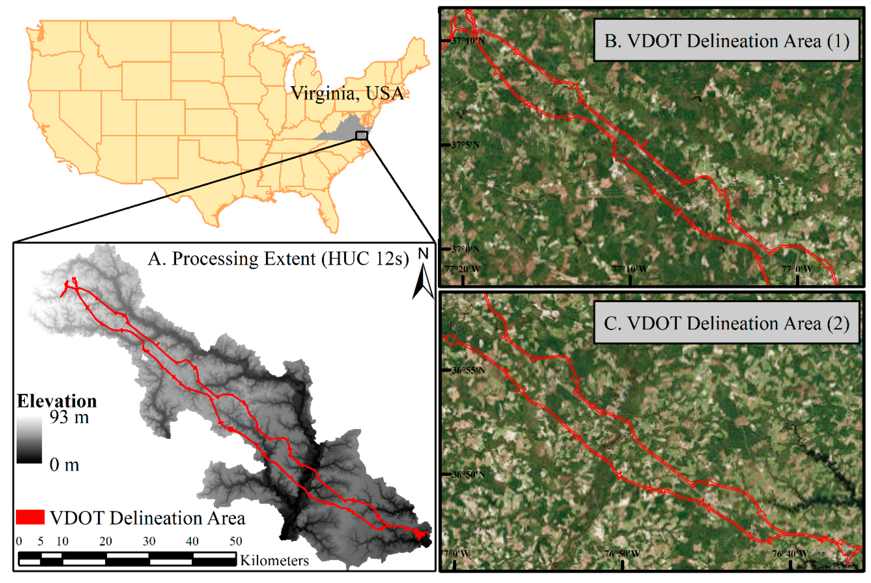
2.1. Study Area

The study area is in the Hampton Roads region of Virginia and is defined by the 33 km² limits of Virginia Department of Transportation (VDOT) wetland delineations and the 1363 km² processing extent encompassing delineations (Figure 1). The processing extent was defined by the 12-digit hydrologic unit codes (HUC 12s), unique identifiers for watersheds in the U.S. [30] (Figure 1A), that were intersected by the VDOT delineations (Figure 1B,C). The study area resides within the Mid-Atlantic Coastal Plain ecoregion. The Mid-Atlantic Coastal Plain is characterized by primarily flat topography and poorly drained soils, and the characteristic land cover includes forest, agriculture, and wetlands [31]. According to the VDOT delineations, wetlands are widespread throughout the area with a wetland to non-wetland ratio of 0.4.

2.2. Input Data and Preprocessing

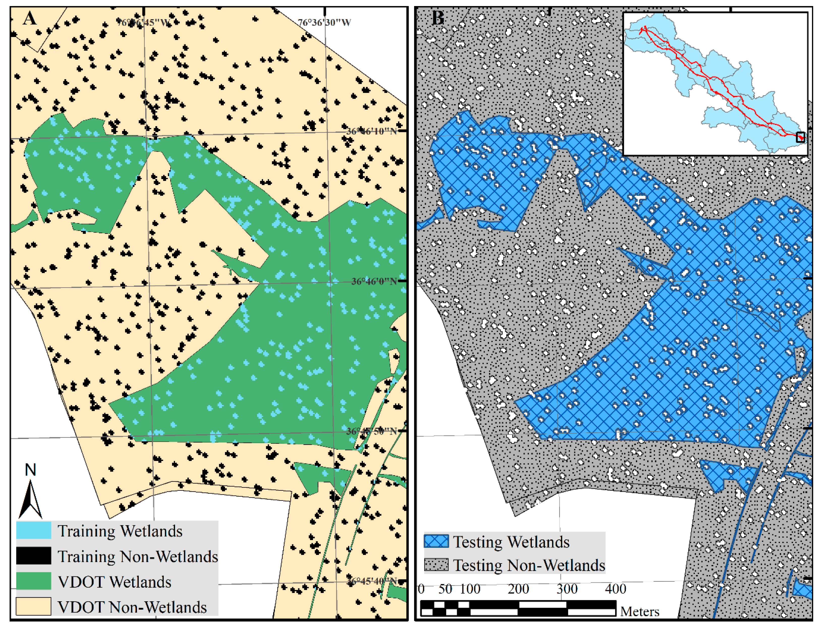
2.2.1. Wetland Delineations (Training and Testing Data)

Wetland delineations obtained from VDOT were the only input data used that are not available on a national scale. Similar data would be required to apply the methodology for different regions. The wetland delineations were produced through field surveys completed for a corridor project and were provided in polygon vector format. Field surveys were conducted by professional wetland scientists during the period of May–July of 2013 and 2015, and were jurisdictionally confirmed by the USACE. These data were considered to be ground truth given their creation through manual surveying by trained analysts and subsequent confirmation of the delineations by the governing authority in wetland permitting. The delineated wetlands were originally categorized by wetland type and included emergent wetlands, forested wetlands, open water, scrub/shrub wetlands, and unconsolidated bottom wetlands. However, all types were generalized into a single “wetland” class, as the wetland screening tool was configured to detect characteristics shared by all wetland types to provide a first order nomination of likely wetland areas.

The delineations were randomly split into two different datasets, a training dataset and a testing dataset, with the majority of wetlands as testing data, as is typically done for building classification models. The training dataset, which included 10% of the delineated wetland area, was used to create the classification model. The testing dataset, which included the remaining 90% of the total wetland area, was used to evaluate the accuracy of the classification model. To create the training dataset, stratified random points were generated among the wetland and non-wetland classes, spanning the entirety of the delineated area. These points were then buffered to encompass 100 m² each and assigned wetland and non-wetland values on a per-pixel basis, according to the underlying delineation information. These processes resulted in a randomly dispersed training dataset with class proportions that are representative of the true land cover, as suggested by Millard and Richardson [22]. Figure 2 shows a portion of the training (A) and testing (B) datasets and

Table 1. Distribution of wetland and non-wetland areas within the VDOT delineations, training dataset, and testing dataset. Randomly selected 10% and 90% portions of VDOT delineations were used to create training and testing data, respectively, and these data maintain land class proportions that are representative of the true land cover, according to VDOT delineations.

	Total Area (km2)	Wetlands (km2)	Non-Wetlands (km2)	Wetland to Non-Wetland Ratio
VDOT Delineations	33.0	8.8	24.2	0.4
Training Data	3.0	0.8	2.2	0.4
Testing Data	30.0	8.0	22.0	0.4

provides further details describing the entirety of the data.

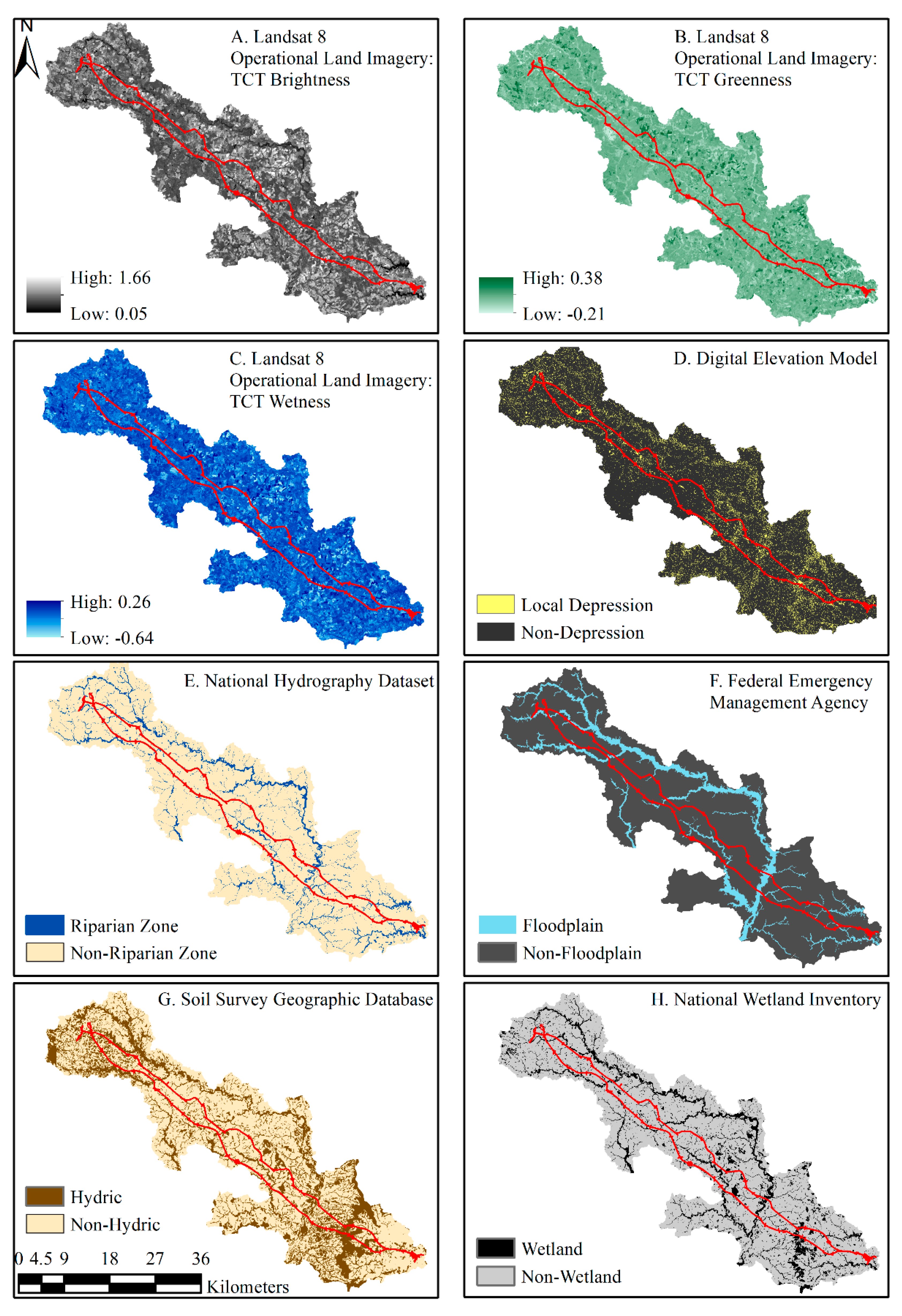
2.2.2. National-Scale Data

Digital Elevation Models (DEMs) were used to derive regions where there is a high likelihood for pooled water, high soil moisture, and, therefore, probable wetland areas. Elevation data were obtained from the U.S. Geological Survey (USGS) National Map Download Client [32] in raster format. The highest available resolution tiles included 1/9th (~3 m) and 1/3rd arc-second (~9 m) data [33]. The vertical accuracy of these data can vary significantly across the United States, but is estimated to be around 1.5 m root mean squared error for the entire conterminous United States [34]. The 1/3rd arc-second DEM tiles covered approximately 300 km² of the processing extent and were resampled using the bilinear resampling technique to match the 1/9th arc-second resolution. As the DEM data provided the highest resolution information, 3 m was used as the pixel size for all subsequent vector to raster conversion and resampling of coarser rasters.

Multispectral imagery from the Landsat 8 OLI satellite was used to detect optical and vegetative wetland characteristics. Data were acquired from the USGS Earth Explorer in raster format with a 30 m resolution [35]. Imagery was chosen that provided cloud-free, spring conditions, as done by researchers in similar Coastal Plains studies (e.g., [12,23,36]), and that was collected on dates near the creation of VDOT delineations. The Landsat scene selected was collected on 4 April 2016 with 4.0% cloud cover. The date of 4 April was selected because, being the early spring season in Virginia, it is likely to have high soil moisture conditions. Visual analyses showed there was no cloud cover over the training and testing areas. Imagery preprocessing included conversion to top of atmosphere reflectance, according to USGS guidelines [37], and pixel resampling.

Federal Emergency Management Agency (FEMA) floodplain maps were used to identify areas of water inundation for heavy storm or flood events. FEMA 100-year floodplain maps are generated at a 1:12,000 scale and were downloaded from the FEMA Flood Map Service Center in polygon vector format [38]. All flood zones designated as 1-percent annual chance flood zones [39] were merged to create the 100-year floodplain zone for the study area. These data showed that floodplains occupy approximately 160 km² (12%) of the processing extent and 1.6 km² (5%) of the VDOT delineations. There were no significant cases of categorical maps spatially conflicting during the merging process.

Soil Survey Geographic Database (SSURGO) soil data, available through the United States Department of Agriculture (USDA), provided information on the location of hydric soils, which are characteristic of wetlands. Hydric soils are defined as soil that is formed under conditions of saturation, flooding, or ponding long enough during the growing season to develop anaerobic conditions in the upper horizon [6]. SSURGO maps are generated at a 1:12,000 scale and were downloaded in polygon vector format from the Natural Resources Conservation Service’s Web Soil Survey [40]. According to SSURGO data, there are approximately 410 km² of hydric soils within the processing extent (30% of area) and 9 km² within the VDOT delineations (27% of area). There were no significant cases of categorical maps spatially conflicting during the merging process.

In addition to providing information on HUC 12 boundaries, national-scale hydrography data were used to estimate riparian zones. Riparian areas are lands that occur along flow channels and waterbodies, and most riparian areas either meet the Cowardin criteria for wetlands, which is a commonly used wetland classification system [5], or share many characteristics and functions with wetlands [41]. To estimate riparian boundaries, streams and waterbodies were downloaded from the National Hydrography Dataset (NHD). Streams used in this study consisted of NHD flowlines, in polygon vector format, categorized as stream/rivers, artificial paths, and connectors. Waterbodies used in this study consisted of NHD waterbodies, in polygon vector format, categorized as swamps/marshes, lakes/ponds, and reservoirs. Both datasets were obtained using the USGS National Map Download Client at a 1:24,000 map scale [32]. According to these data, there are approximately 1030 km of streams and 67 km² of waterbodies within the processing extent (5% of area) and 16 km of streams and 0.5 km² of waterbodies within VDOT delineations (1.5% of area).

Land cover data were used to identify certain land cover types where wetlands may be more likely to occur. These data were downloaded from the 2011 National Land Cover Database (NLCD) in raster format from the USGS National Map Download Client [32]. NLCD data were resampled from 30 m resolution to match that of the DEM using the majority resampling technique.

Table 2. Summarized land cover class distribution for the processing extent (left) and VDOT delineated area (right) according to the 2011 NLCD [42].

Land Classification	Processing Extent		VDOT Delineated Area
	Area (km2)	Percent Area	Area (km2)	Percent Area
Barren Land	6.52	0.5	0.15	0.5
Developed	110.25	8.1	6.85	20.8
Forest	466.59	34.2	10.61	32.2
Grassland	40.87	3.0	0.76	2.3
Open Water	10.30	0.8	0.04	0.1
Cropland	340.00	25.0	7.68	23.3
Shrub	164.35	12.1	3.65	11.1
Wetlands	223.62	16.4	3.24	9.8
∑=	1362.5	-	33.0	-

provides the summarized distribution of NLCD classes within the processing extent (left) and VDOT delineated area (right). Note that although the NLCD data include a wetland category, these areas refer to the NWI wetland designations.

Lastly, NWI wetlands were included in the wetland tool workflow under the assumption that the NWI is incomplete rather than incorrect. NWI maps are generated at a 1:24,000 scale and were downloaded from the USFWS in polygon vector format [43]. According to the NWI, there are approximately 200 km² of wetlands within the processing extent (15% of area) and 3 km² within the VDOT delineations (9% of area).

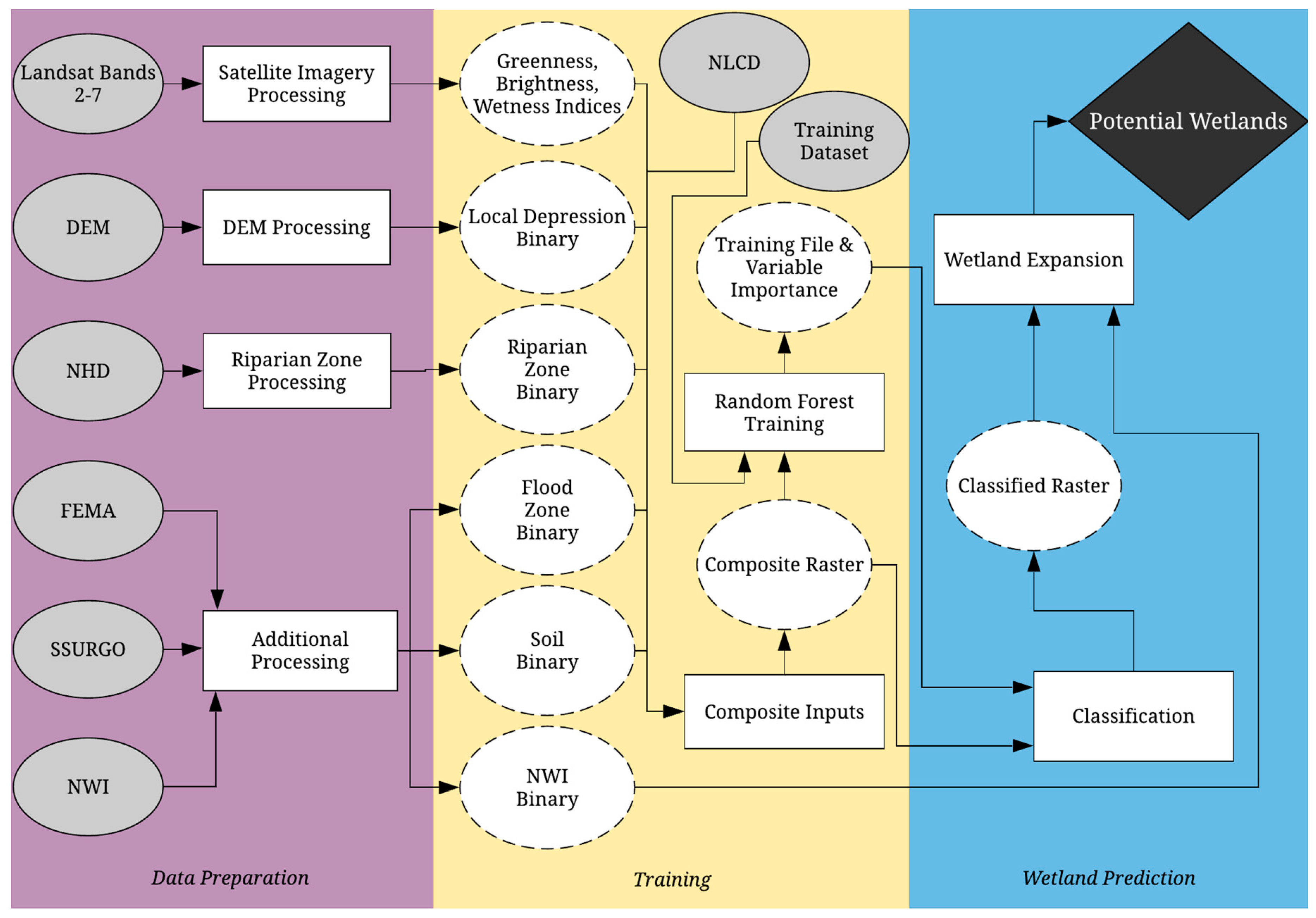
2.3. Screening Methodology Design and Implementation

The wetland screening methodology can be described as a workflow (Figure 3) that was implemented within ArcGIS 10.4 using their Model Builder tool. The workflow is segmented into three main sections, data preparation, training, and wetland prediction, each of which is described in detail in the following subsections. Implementing the methodology as a workflow within Model Builder allows it to be executed as a succession of geoprocessing and analysis tools able to transform nationally available data to potential wetlands maps with minimal user intervention. We selected Model Builder as the platform for implementation because (i) ArcGIS is a widely used software system within VDOT and likely other state DOTs as well, (ii) the graphical user interface (GUI) provides end users with workflow transparency, and (iii) workflows in this system can be exported to the Python programming language for further enhancement and automation.

2.3.1. Data Preparation

Data preparation includes satellite imagery processing, DEM processing, riparian zone processing, and additional processing. The methodology for executing these processes is given below and the results of each process are shown in Figure 4.

The satellite imagery processing consists of performing a Tasseled Cap Transformation (TCT) on the Landsat 8 OLI bands 2–7. The TCT is used to reduce dimensionality from several bands to a few bands associated with physical scene characteristics; specifically, brightness, greenness, and wetness, which are calculated as

$$\mathrm{B}\mathrm{r}\mathrm{i}\mathrm{g}\mathrm{h}\mathrm{t}\mathrm{n}\mathrm{e}\mathrm{s}\mathrm{s}={\displaystyle \sum }_{i=2}^7(w_{1i}\times ban{d}_i)$$

(1)

$$\mathrm{G}\mathrm{r}\mathrm{e}\mathrm{e}\mathrm{n}\mathrm{n}\mathrm{e}\mathrm{s}\mathrm{s}={\displaystyle \sum }_{i=2}^7(w_{2i}\times ban{d}_i)$$

(2)

$$\mathrm{W}\mathrm{e}\mathrm{t}\mathrm{n}\mathrm{e}\mathrm{s}\mathrm{s}={\displaystyle \sum }_{i=2}^7(w_{3i}\times ban{d}_i)$$

(3)

where $w$ is a scalar used for weighing bands (

Table 3. Tasseled cap transformation (TCT) coefficients for the Landsat 8 Operational Land Imagery (OLI) bands derived by Baig et al. [44].

Landsat 8 OLI	Blue	Green	Red	NIR	SWIR1	SWIR2
TCT	Band 2	Band 3	Band 4	Band 5	Band 6	Band 7
Brightness	0.3029	0.2786	0.4733	0.5599	0.5080	0.1872
Greenness	−0.2941	−0.2430	−0.5424	0.7276	0.0713	−0.1608
Wetness	0.1510	0.1973	0.3283	0.3407	−0.7117	−0.4559

), derived by Baig et al. [44]. Brightness measures are related to soil and albedo, greenness describes the presence of vegetation, and wetness describes water content [44]. Panels A, B, and C of Figure 4 show the resulting brightness, greenness, and wetness rasters, respectively.

The DEM processing creates a binary local depression raster. The DEM is first conditioned using rasterized NHD streams with a 3 m resolution, per the DEM raster constraints. The DEM is artificially lowered by a large depth, in this case 100 m, where NHD raster pixels exist by executing the Map Algebra Expression (4).

Con (IsNull (Stream Raster)), DEM, (DEM − 100))

(4)

resulting in the reconditioned streams DEM. After Expression (4) is executed, local depressions are filled using the Planchon and Darboux method [45]. This operation is generally used to remove small imperfections or barriers in topography for hydrologic flow path analysis; however, here it is used to identify areas of local depressions that could indicate wetlands in the low relief topography. Local depressions (Figure 4D) are identified by flagging differences in the filled reconditioned stream (FRS) DEM compared to the original DEM using the Map Algebra Expression (5).

Con (FRS DEM == DEM, 0, 1)

(5)

The riparian zone processing creates a binary riparian zone raster. As previously described, riparian areas are located along waterbodies and often exhibit wetland characteristics; however, riparian extents surrounding waterbodies can vary significantly, and there is no single agreed upon buffer distance to encompass riparian zones [41]. Here, practices associated with Virginia riparian zone policies, in the context of best management practices for water quality purposes, were analyzed to estimate a standard buffer width. The Chesapeake Bay Agreement recognizes a 15 m (50 ft) wide vegetative buffer extending from theoretical centerlines as forested riparian areas, enforced in lands within the Coastal Plains portion of the Chesapeake Bay watershed [46]. Thus, a 15 m buffer width extending from each side of NHD streams and waterbodies was used to represent the riparian zone, similar to the practice used by Hancock et al. [47]. The resulting polygon vector dataset was rasterized with the 3 m pixel resolution constraint and assigned values corresponding to either within or outside of the riparian zone (Figure 4E).

In additional processing, binary rasters were created for FEMA, SSURGO, and NWI datasets. A binary floodplain raster is created where pixels within the 100-year floodplain are set to a value of one, and all other areas are set to a value of zero (Figure 4F). A binary soil raster is created where pixels containing hydric soils are set to a value of one and pixels containing non-hydric soils are set to a value of zero (Figure 4G). A binary NWI raster is created where pixels within wetland areas are set to a value of one and pixels within non-wetland areas are set to a value of zero (Figure 4H). NLCD data are incorporated without additional processing.

2.3.2. Training

The training portion of the workflow involves two processes: composite inputs and random forest training. In the composite inputs process, the tool combines all prepared input data, with the exception of NWI data, into a multiband raster where each band stores the attributes of a single input. In the random forest training process, the composite raster and the training dataset are used as inputs to the Train Random Trees tool to extract wetland and non-wetland signatures. Train Random Trees executes the OpenCV implementation of the random forest algorithm within the ArcGIS environment [48]. This process also produces measures of variable importance based on the mean decrease in accuracy when a variable is not used in generating a tree [20]. The Train Random Trees tool allows users to specify values for the maximum number of trees, maximum tree depth, and maximum numbers of samples per class [49]. For this preliminary demonstration of the tool, these values were held constant at the ArcGIS recommended values of 50, 30, and 1000, respectively.

2.3.3. Wetland Prediction

The wetland prediction section includes classification and wetland expansion. During classification, the Classify Raster tool uses training information to classify the entire composite raster. The result of this operation is a binary wetland raster. In the wetland expansion section, a final tool output of the potential wetland raster is created by merging the classified wetlands with the NWI wetlands. As previously noted, NWI wetlands should not be the sole source for wetland screening; however, here NWI data are used to expand the classified wetland class in the interest of meeting the tool’s objective to screen for areas where wetlands are likely to occur. The binary NWI raster is used to supplement classification results by applying the Map Algebra Expression (6).

Con (NWI binary == 0, 0, classified raster)

(6)

Executing this expression results in a binary final potential wetlands raster.

2.3.4. Accuracy Assessments

Accuracy assessments were performed using a confusion matrix summarizing only predicted areas in the testing dataset that were not used for training. In each confusion matrix, testing data are represented along columns and either the screening tool (A) or NWI (B) data are represented along rows. Wetland tool and NWI performance were defined in terms of false negative rate, false positive rate, and overall accuracy. The false negative rate represents the tendency of models to omit true wetlands, and is defined as Equation (7).

$$\mathrm{F}\mathrm{a}\mathrm{l}\mathrm{s}\mathrm{e}\mathrm{n}\mathrm{e}\mathrm{g}\mathrm{a}\mathrm{t}\mathrm{i}\mathrm{v}\mathrm{e}\mathrm{r}\mathrm{a}\mathrm{t}\mathrm{e}=\frac{\mathrm{F}\mathrm{a}\mathrm{l}\mathrm{s}\mathrm{e}\mathrm{n}\mathrm{o}\mathrm{n}\mathrm{w}\mathrm{e}\mathrm{t}\mathrm{l}\mathrm{a}\mathrm{n}\mathrm{d}\mathrm{p}\mathrm{r}\mathrm{e}\mathrm{d}\mathrm{i}\mathrm{c}\mathrm{t}\mathrm{i}\mathrm{o}\mathrm{n}\mathrm{s}}{\mathrm{T}\mathrm{o}\mathrm{t}\mathrm{a}\mathrm{l}\mathrm{w}\mathrm{e}\mathrm{t}\mathrm{l}\mathrm{a}\mathrm{n}\mathrm{d}\mathrm{s}}$$

(7)

The false positive rate represents the tendency of models to overpredict wetlands and is defined as Equation (8).

$$\mathrm{F}\mathrm{a}\mathrm{l}\mathrm{s}\mathrm{e}\mathrm{p}\mathrm{o}\mathrm{s}\mathrm{i}\mathrm{t}\mathrm{i}\mathrm{v}\mathrm{e}\mathrm{r}\mathrm{a}\mathrm{t}\mathrm{e}=\frac{\mathrm{F}\mathrm{a}\mathrm{l}\mathrm{s}\mathrm{e}\mathrm{w}\mathrm{e}\mathrm{t}\mathrm{l}\mathrm{a}\mathrm{n}\mathrm{d}\mathrm{p}\mathrm{r}\mathrm{e}\mathrm{d}\mathrm{i}\mathrm{c}\mathrm{t}\mathrm{i}\mathrm{o}\mathrm{n}\mathrm{s}}{\mathrm{T}\mathrm{o}\mathrm{t}\mathrm{a}\mathrm{l}\mathrm{n}\mathrm{o}\mathrm{n}\mathrm{w}\mathrm{e}\mathrm{t}\mathrm{l}\mathrm{a}\mathrm{n}\mathrm{d}\mathrm{s}}$$

(8)

Overall accuracy, Equation (9), represents the ability of models to correctly classify the total testing area, regardless of class.

$$\mathrm{O}\mathrm{v}\mathrm{e}\mathrm{r}\mathrm{a}\mathrm{l}\mathrm{l}\mathrm{a}\mathrm{c}\mathrm{c}\mathrm{u}\mathrm{r}\mathrm{a}\mathrm{c}\mathrm{y}=\frac{\mathrm{T}\mathrm{r}\mathrm{u}\mathrm{e}\mathrm{w}\mathrm{e}\mathrm{t}\mathrm{l}\mathrm{a}\mathrm{n}\mathrm{d}\mathrm{p}\mathrm{r}\mathrm{e}\mathrm{d}\mathrm{i}\mathrm{c}\mathrm{t}\mathrm{i}\mathrm{o}\mathrm{n}\mathrm{s}+\mathrm{T}\mathrm{r}\mathrm{u}\mathrm{e}\mathrm{n}\mathrm{o}\mathrm{n}\mathrm{w}\mathrm{e}\mathrm{t}\mathrm{l}\mathrm{a}\mathrm{n}\mathrm{d}\mathrm{p}\mathrm{r}\mathrm{e}\mathrm{d}\mathrm{i}\mathrm{c}\mathrm{t}\mathrm{i}\mathrm{o}\mathrm{n}\mathrm{s}}{\mathrm{T}\mathrm{o}\mathrm{t}\mathrm{a}\mathrm{l}\mathrm{p}\mathrm{r}\mathrm{e}\mathrm{d}\mathrm{i}\mathrm{c}\mathrm{t}\mathrm{e}\mathrm{d}\mathrm{a}\mathrm{r}\mathrm{e}\mathrm{a}}$$

(9)

Note that the false positive rate is equivalent to one minus the true negative rate, and the false negative rate is equivalent to one minus the true positive rate (i.e., the producer’s accuracy). In addition, the Kappa statistic [50], which quantifies model performance taking into account the estimated performance of a random classifier, was also used to compare the wetland tool and NWI output. This set of performance criteria is not exhaustive but is appropriate to evaluate the testing area given the nearly balanced true wetland and true non-wetland classes [51].

3. Results

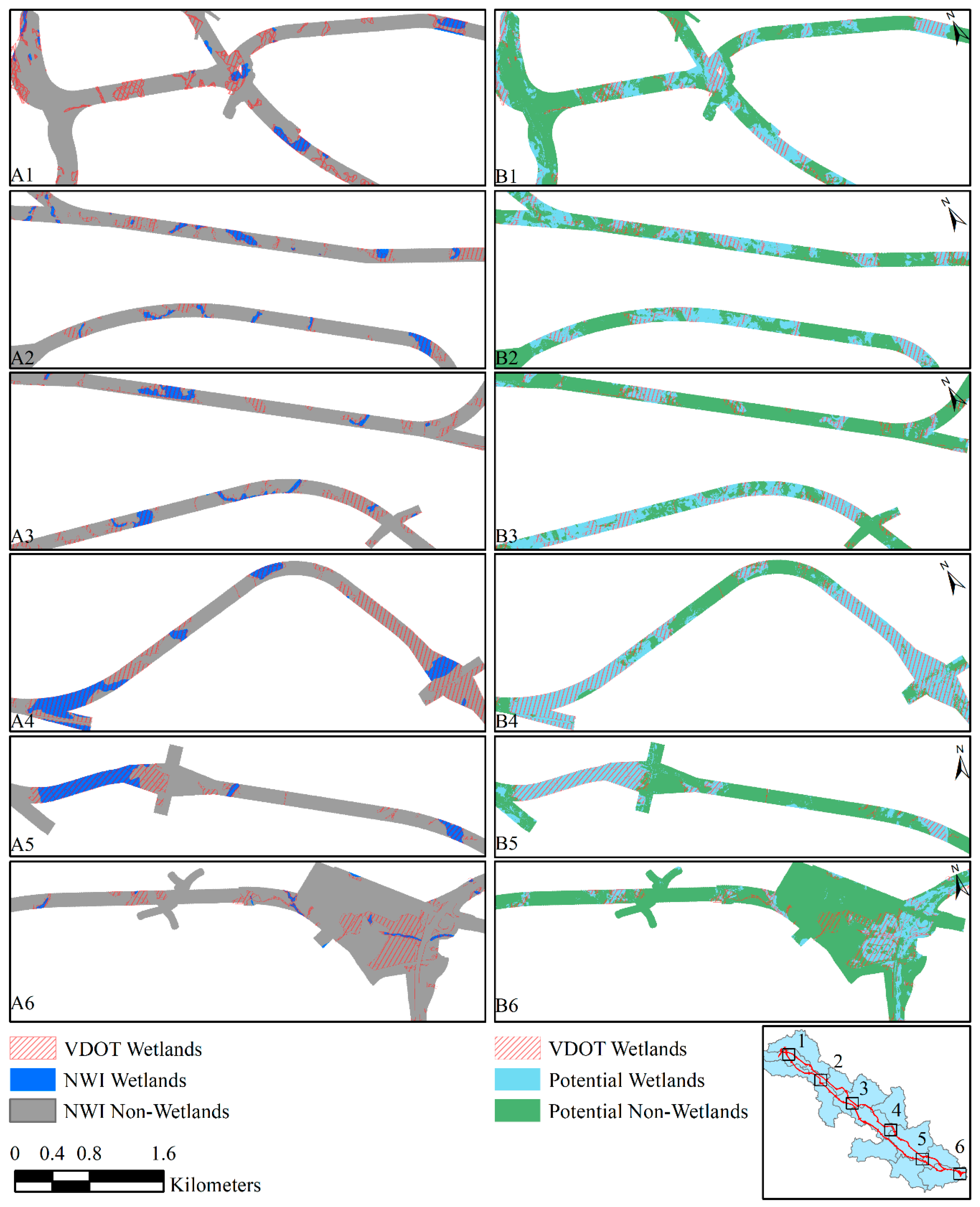
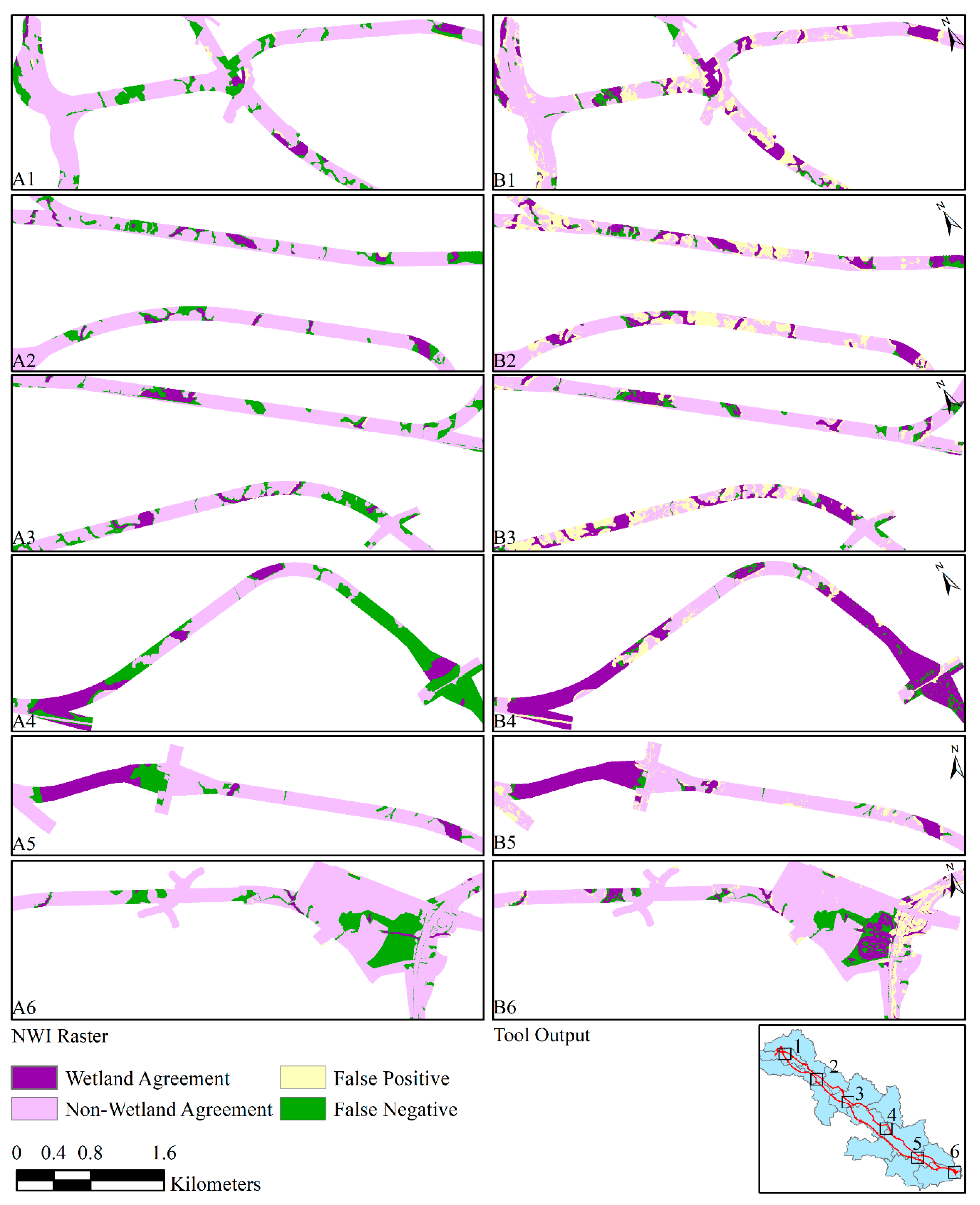
3.1. Screening Method Results Compared to the NWI

Figure 5 shows the comparison between our screening tool predicted wetlands and NWI-designated wetlands for several areas within the larger study region. The “ground-truth” wetland delineations obtained by VDOT are included for reference. The levels of agreement between both wetland maps and VDOT delineations are represented as either wetland agreement, non-wetland agreement, false positive, or false negative in Figure 6. Note that scenes in Figure 5 and Figure 6 include both training and testing locations (i.e., the entirety of the VDOT delineated area) for clarity, although only testing locations are included in performance assessments. In Figure 5, NWI maps show a tendency to underestimate VDOT wetlands, represented by relatively large distributions of false negative predictions in Figure 6. This trend is especially prominent in scene A6, where nearly all VDOT wetlands are missed by the NWI. Figure 5 scenes also demonstrate that in instances where NWI wetlands are correct, NWI wetland boundaries align relatively precisely with VDOT wetland boundaries. This trend is translated to significantly smaller distributions of false positive predictions in Figure 6. In contrast, the potential wetland areas predicted by our method more robustly encompass extents of VDOT delineations in scenes B1–B6 of Figure 5. However, the improved coverage of true wetlands was accompanied by imprecise wetland boundaries and wetland overestimation. In scenes B1–B6 of Figure 6, the wetland screening tool results in both larger areas of wetland agreement and false positive predictions surrounding predicted wetlands, relative to NWI mapping results.

3.2. Confusion Matrix

The confusion matrix resulting from the classification tool testing (

Table 4. Confusion matrices used to assess the accuracy of screening tool predictions (A) and the NWI raster (B), where testing data classes are represented in columns and both tool and NWI classes are represented in rows. Both accuracy assessments quantify the level of agreement achieved by respective datasets within the limits of the testing dataset.

A
Screening Tool Prediction Classes	Testing Data Classes
	Wetland (km2)		Non-Wetland (km2)	∑ =
Wetland (km2)	6.16		5.32	11.5
Non-Wetland (km2)	1.80		16.55	18.4
∑ =	8.0		21.9	30
Overall Accuracy = 76.1%		Kappa Statistic = 0.46
False Positive Rate = 24.3%		False Negative Rate = 22.6%
B
NWI Raster Classes	Testing Data Classes
	Wetland (km2)		Non-Wetland (km2)	∑ =
Wetland (km2)	2.45		0.28	2.7
Non-Wetland (km2)	5.53		21.62	27.1
∑ =	8.0		21.9	30
Overall Accuracy = 80.5%		Kappa Statistic = 0.34
False Positive Rate = 1.3%		False Negative Rate = 69.3%

) shows that the screening tool produced a higher kappa statistic (0.46 vs. 0.34, respectively) and predicted 76.1% of the total testing area correctly, whereas the NWI correctly predicted 80.5% of the same area. Focusing more specifically on wetland prediction rates, the screening tool omitted 22.6% of wetlands from the testing dataset in its predictions, compared to 69.3% of the testing wetlands being missed by NWI maps. However, the screening tool incorrectly included 24.3% of testing nonwetland area in wetland predictions, whereas the NWI maps misidentified only 1.3% of the nonwetland area. These statistics are in line with trends observed in Figure 5 and Figure 6, where the wetland screening tool encompassed more of the true wetland area while also over estimating the distribution and extents of VDOT wetlands. This assessment shows that, when used as a preliminary screening tool, it is expected that the method would identify 77.4% of wetlands (one minus the false negative rate) and 24.3% of non-wetland area would be unnecessarily surveyed (per the false positive rate). In contrast, using solely the NWI as a preliminary estimate of wetlands, only 30.7% of wetlands would be identified and 1.3% of the nonwetland area would be unnecessarily surveyed. Given that missing wetland areas can have significant consequences in the LEDPA environmental planning process, these statistics illustrate the potential benefit of using this wetland screening tool, along with targeted wetland identification by experts, compared to relying solely on NWI in the LEDPA process.

4. Discussion

4.1. Ecohydrologic Insights into the Method Performance

Understanding the underlying ecohydrologic properties of the study region and how they influence the method’s performance is useful for guiding future efforts to improve the method. Scene B6 of Figure 5 and Figure 6 shows a relatively large distribution of false negative predictions. Investigation of the input data in this area shows that wetland omission may be due to the presence of non-wetland characteristics, including low TCT wetness values, scattered distributions of small local depressions and small hydric soil areas, location outside of floodplains, location outside of riparian zones, and mostly developed NLCD classification. It is possible that wetland characteristics are present on a finer scale here, but the current resolution of wetland indicators resulted in overly generalized boundaries between heterogeneous areas. In addition, VDOT wetlands in this area may be the result of data not included in the screening tool like groundwater levels, which are important in this region but difficult to quantify due to limited observational data. In addition, higher resolution topographic inputs that take into account slope, curvature, and flow accumulation have been found to successfully capture wetland hydrology (e.g., [24,52,53,54,55,56,57,58,59]) and may improve approximation of saturated areas at a finer resolution. Similar studies have shown that finer-scale multispectral imagery would better distinguish detailed boundaries between developed areas and vegetation types (e.g., [16,17,19]), which would be especially important for identifying wetlands close to developed structures.

Although secondary to false negative rate, maintaining a low false positive rate is also important to creating a trustworthy screening tool. Scene B2 of Figure 5 and Figure 6 demonstrates problematic false positive predictions by the screening tool. The input data here show widespread distributions of hydric soils and local depressions, both of which are likely to have contributed to wetland predictions. Disagreement between these predictions and VDOT wetlands could likely be related to overly generalized landscape due to coarse input data, as described above. However, false positive predictions that are adjacent to and surround correct wetland predictions may represent difficulty in assigning definitive extents to seasonally fluctuating wetland boundaries. While the Landsat-derived inputs generally represent the seasonal characteristics inherent to the VDOT delineations, other inputs can be considered time-averaged wetland indicators. Information from these input data likely contribute to screening tool predictions in the correct general area but with imprecise boundaries, as the true wetland boundaries are diffuse and season-dependent.

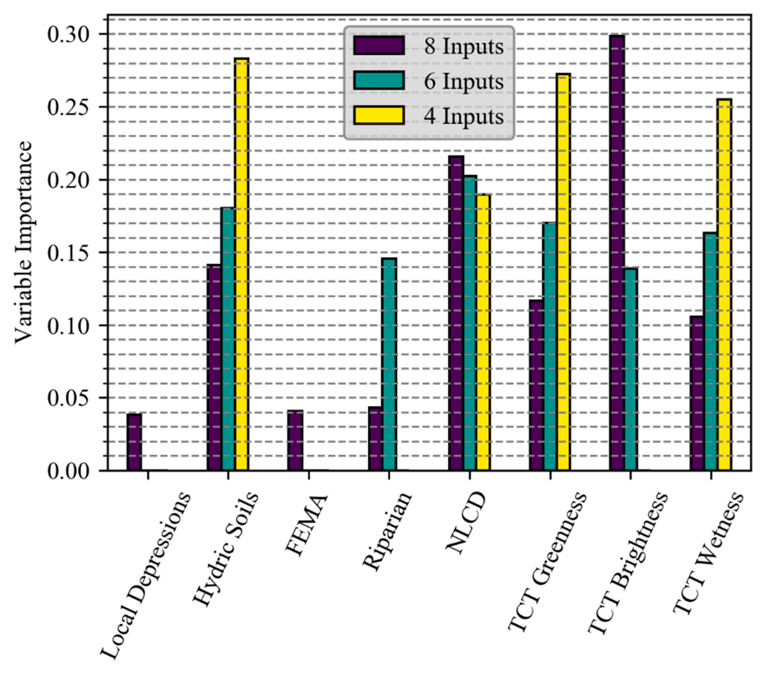
4.2. The Importance of Variable Inputs

Variable importance measures were used to investigate the value of the multisource input dataset. These measures can help target future efforts in refining the datasets most important to the wetland screening methodology. Figure 7 shows the variable importance measures for the proposed eight-input classification (classification 1), as well as measures for execution using the six most important inputs from classification 1 (classification 2) and the four most important inputs from classification 2 (classification 3).

Figure 7 shows that TCT brightness and greenness were among the most important input variables in each classification. These indices have also been found to be key input variables in multisource datasets used to identify wetlands in similar studies (e.g., [23,60]). Here, it is expected that TCT brightness and greenness were consistently important wetland indicators as they provide vegetative and optical characteristics that are also seasonally representative of the VDOT delineations. Since these data are derived from Landsat imagery, it is important to select Landsat images that provide ideal conditions for wetland classification. As stated in the introduction, this means spring conditions with high soil moisture and cloud cover are minimal. Without these conditions, it is possible that the method will be unable to accurately identify potential wetland locations. The importance of the hydric soils input was also consistently high, which has been observed in related studies as well (e.g., [24,60]). While it was expected that hydric soils would be successful indicators of wetlands as they are included in the wetland criteria, this trend shows that SSURGO hydric soil information was useful at our target scale despite the relatively coarse resolution of these data. The low importance of the local depressions input was unexpected since this layer was intended to indicate areas where water is likely to pool. It is likely that the elevation data used was too coarse to model the low-relief area and that additional topographic metrics would more robustly describe hydrologic drivers of wetland formation.

Additional accuracy assessments were performed for classifications 2 and 3 and are shown with the classification 1 assessment in

Table 5. Accuracy rates achieved as a result of varying input variables in classifications 1, 2 and 3.

Classification	Overall Accuracy (%)	False Negative Rate (%)	False Positive Rate (%)
1	76.1	22.6	24.3
2	74.3	22.3	26.9
3	73.2	26.6	26.9

. The accuracy assessments show that overall accuracy decreases consistently as input variables were removed from the workflow. In addition, false positive rates increase and false negative rates are variable. The overall accuracy trend shows that the screening tool is overall better able to distinguish between wetlands and non-wetlands given information from the eight originally proposed input variables. The increasing false positive rates suggest that local depressions, floodplains, riparian areas, and TCT brightness provided important information that contribute to correct non-wetland designations. Despite the false negative rate decreasing by a small margin between classifications 1 and 2, the overall higher false negative rate in classification 3 demonstrates the ability of the larger input set to capture a more robust set of wetland characteristics. It is important to note, however, that accuracy rates shown in Table 5 varied only slightly, which suggests that some of the input data provide similar spatial information, and therefore there is a relatively small cost to the accuracy when one of these layers is removed.

4.3. Potential for Additional Data and Tool Improvements

While there are several ways to advance the wetland screening method presented here, improving the quality of the input data is an important next step. In particular, using higher resolution topographic data would likely improve results. To maintain the goal of using data generally available at a national-scale, incorporating higher resolution elevation data would be the most viable next step as Light Detection and Ranging (LiDAR) elevation data is quickly growing in availability [53]. Furthermore, the ability to model small topographic changes through data products easily derived from digital elevation models (DEMs) would be particularly useful in mapping saturated areas in the low-relief terrain studied here. If high resolution multispectral imagery becomes widely available, this would also be a valuable addition to the improved wetland screening tool and may present potential for distinguishing between different classes of wetlands. Moreover, radar data may contribute additional vegetative information that is helpful for wetland mapping, as demonstrated by researchers (e.g., [23,26,61,62]). Also regarding the quality of input data, the riparian zone can be estimated in a more sophisticated way. The application of a standard riparian distance to all waterbodies could be improved by instead using variable riparian buffer distances based on the size of waterbodies and bank geomorphology, as suggested by other studies [15,24].

Additional field-verified wetland maps used to train the model and quantify its error could be obtained for other areas. Including more training data from other study areas would likely improve the robustness of wetland and non-wetland signatures detected by the random forest model. Further analysis would likely benefit the procedure used to determine the optimal train-test split of these delineated wetland areas to determine when diminishing returns of accuracy begin as more of the area is used for training. Given the unequal distribution of wetland to nonwetland area in this study region, and likely other regions as well, further work to optimize the sampling scheme between wetland and nonwetland classes of the training data, which has been shown to significantly impact wetland classifications [22], is another area for improvement.

Lastly, reconfiguring the workflow to execute using open source Python libraries would offer several advantages. Open source geoprocessing libraries such as GRASS GIS [63], GDAL [64], and TauDEM [65] would allow users without an ArcGIS license to execute necessary processes. Additionally, Scikit-Learn [66] implementation of random forest would offer more flexibility than the ArcGIS implementation in terms of random forest parameters. Following this, analyses for random forest parameter tuning should be performed to test if moving from the standard configuration for parameters improves classification accuracy.

5. Conclusions

This study presents a methodology designed to screen for wetlands over a large geographic region using nationally available geospatial data as input and random forest classification. The methodology was motivated by the desire to streamline environmental permitting for transportation corridor projects over large regions. By using a tool to screen for potential wetland areas, field surveying efforts could be focused to areas that are likely to contain wetlands. The methodology was implemented as an automated workflow in a commercially available geographic information system (GIS) software commonly used by DOTs. The tool was applied to identify potential wetland locations for a region in the coastal plain of Virginia, USA. The preliminary implementation of this workflow was evaluated against professionally conducted field surveys and results were compared to the commonly used NWI dataset as a benchmark for accuracy.

Results showed that, when compared to the NWI, the wetland screening methodology produced a significantly lower false negative rate (22.6% vs. 69.3%) and a higher kappa statistic (0.46 vs. 0.34). From this, we conclude that the methodology was able to capture many wetlands missed by NWI. However, this improvement in false negative predictions did result in a higher false positive rate (24.3% vs. 1.3%) and, because the study area has more non-wetland area, a slightly lower overall accuracy (76.1% vs. 80.5%). From this, we conclude that, while the method identifies significantly more true wetlands than the NWI, it comes at the cost of a slight reduction in overall prediction accuracy. This was largely by design, however, as the method purposely avoids false positives because such errors would result in missing wetlands and be costly in environmental planning. False negative errors are less costly because they could be field verified by targeted, on-the-ground surveys by experts to fine tune the wetland delineation. With additional wetland areas mapped and verified by experts, the method could be tested for other regions given that, by design, it only relies on nationally available input datasets.

While successful as a screening tool, the ultimate goal should be to achieve the highest possible overall classification accuracy at a spatial scale relevant for environmental planning purposes. Doing so would move the approach from being a wetland screening tool to a wetland mapping tool, opening up additional potential uses. For example, because the approach is largely automated now, future work could also investigate the potential for deriving time varying wetland maps using Landsat imagery and a dynamic input to capture change in wetland patterns across regions. Making this transition will likely require much higher resolution data and more data for training classification algorithms. The wetland detection rate produced by the current screening algorithm, which again only makes use of nationally available geospatial data in order to be widely applicable, is encouraging for creating approaches able to identify wetlands at a high resolution. Future work should investigate the role of higher resolution input data, like LiDAR, and alternative parameterizations of the classification algorithm to improve wetlands predictions.

References

1. Klemas, V. Remote Sensing of Wetlands: Case Studies Comparing Practical Techniques. J. Coast. Res. 2011, 27, 418–427. [Google Scholar] [CrossRef]
2. Dahl, T.E. Status and Trends of Wetlands in the Conterminous United States 2004 to 2009; US Department of the Interior, US Fish and Wildlife Service, Fisheries and Habitat Conservation: Washington, DC, USA, 2011.
3. Votteler, T.H.; Muir, T.A. Wetland Protection Legislation; United States Geological Survey, National Water Summary on Wetland Resources: Reston, VA, USA, 1996; pp. 57–64.
4. Page, R.W.; Wilcher, L.S. Memorandum of Agreement Between the Environmental Protection Agency and the Department of the Army Concerning the Determination of Mitigation under the Clean Water Act, Section 404 (b)(1) Guidelines; United States Environmental Protection Agency: Washington, DC, USA, 1990.
5. Cowardin, L.; Carter, V.; Golet, F.; LaRoe, E. Classification of Wetlands and Deepwater Habitats of the United States; U.S. Fish and Wildlife Service: Washington, DC, USA, 1979.
6. Environmental Laboratory. Corps of Engineers Wetlands Delineation Manual; Technical Report Y-8701; U.S. Army Engineer Waterways Experiment Station: Vicksburg, MS, USA, 1987.
7. Tiner, R.W. Use of high-altitude aerial photography for inventorying forested wetlands in the United States. For. Ecol. Manag. 1990, 33, 593–604. [Google Scholar] [CrossRef]
8. NWI Program Overview. Available online: https://www.fws.gov/wetlands/nwi/overview.html (accessed on 30 January 2019).
9. Cowardin, L.M.; Golet, F.C. U.S. Fish and Wildlife Service 1979 wetland classification: A review. Vegetatio 1995, 118, 139–152. [Google Scholar] [CrossRef]
10. Morrissey, L.A.; Sweeney, W.R. Assessment of the National Wetlands Inventory: Implications for wetlands protection. In Proceedings of the Geographic Information Systems and Water Resources IV Awra Spring Specialty Conference, Houston, TX, USA, 8–10 May 2006; pp. 1–6. [Google Scholar]
11. Tiner, R.W. NWI maps: What they tell us. Natl. Wetl. Newsl. 1997, 19, 7–12. [Google Scholar]
12. Kloiber, S.M.; Macleod, R.D.; Smith, A.J.; Knight, J.F.; Huberty, B.J. A Semi-Automated, Multi-Source Data Fusion Update of a Wetland Inventory for East-Central Minnesota, USA. Wetlands 2015, 35, 335–348. [Google Scholar] [CrossRef]
13. Guo, M.; Li, J.; Sheng, C.; Xu, J.; Wu, L. A review of wetland remote sensing. Sensors 2017, 17. [Google Scholar] [CrossRef] [PubMed]
14. Rapinel, S.; Bouzillé, J.-B.; Oszwald, J.; Bonis, A. Use of bi-seasonal Landsat-8 imagery for mapping marshland plant community combinations at the regional scale. Wetlands 2015, 35, 1043–1054. [Google Scholar] [CrossRef]
15. Woodward, B.D.; Evangelista, P.H.; Young, N.E.; Vorster, A.G.; West, A.M.; Carroll, S.L.; Girma, R.K.; Hatcher, E.Z.; Anderson, R.; Vahsen, M.L.; et al. CO-RIP: A Riparian Vegetation and Corridor Extent Dataset for Colorado River Basin Streams and Rivers. ISPRS Int. J. Geo-Inf. 2018, 7, 397. [Google Scholar] [CrossRef]
16. Kaplan, G.; Avdan, U. Monthly Analysis of Wetlands Dynamics Using Remote Sensing Data. ISPRS Int. J. Geo-Inf. 2018, 7, 411. [Google Scholar] [CrossRef]
17. Tian, S.; Zhang, X.; Tian, J.; Sun, Q. Random Forest Classification of Wetland Landcovers from Multi-Sensor Data in the Arid Region of Xinjiang, China. Remote Sens. 2016, 8, 954. [Google Scholar] [CrossRef]
18. Zhu, C.; Zhang, X.; Huang, Q. Four decades of estuarine wetland changes in the Yellow River Delta based on landsat observations between 1973 and 2013. Water 2018, 10, 933. [Google Scholar] [CrossRef]
19. Xiong, D.; Lee, R.; Saulsbury, J.B.; Lanzer, E.L.; Perez, A. Remote Sensing Applications for Environmental Analysis in Transportation Planning: Application to the Washington State I-405 Corridor; WA-RD 593-1; Oak Ridge National Laboratory: Oak Ridge, TN, USA, 2004.
20. Breiman, L. Random forests. Mach. Learn. 2001, 45, 5–32. [Google Scholar] [CrossRef]
21. Rodriguez-Galiano, V.F.; Ghimire, B.; Rogan, J.; Chica-Olmo, M.; Rigol-Sanchez, J.P. An assessment of the effectiveness of a random forest classifier for land-cover classification. ISPRS J. Photogramm. Remote Sens. 2012, 67, 93–104. [Google Scholar] [CrossRef]
22. Millard, K.; Richardson, M. On the importance of training data sample selection in Random Forest image classification: A case study in peatland ecosystem mapping. Remote Sens. 2015, 7, 8489–8515. [Google Scholar] [CrossRef]
23. Corcoran, J.M.; Knight, J.F.; Gallant, A.L. Influence of multi-source and multi-temporal remotely sensed and ancillary data on the accuracy of random forest classification of wetlands in northern Minnesota. Remote Sens. 2013, 5, 3212–3238. [Google Scholar] [CrossRef]
24. O’Neil, G.L.; Goodall, J.L.; Watson, L.T. Evaluating the potential for site-specific modification of LiDAR DEM derivatives to improve environmental planning-scale wetland identification using Random Forest classification. J. Hydrol. 2018, 559, 192–208. [Google Scholar] [CrossRef]
25. Costa, H.; Almeida, D.; Vala, F.; Marcelino, F.; Caetano, M. Land Cover Mapping from Remotely Sensed and Auxiliary Data for Harmonized Official Statistics. ISPRS Int. J. Geo-Inf. 2018, 7, 157. [Google Scholar] [CrossRef]
26. Millard, K.; Richardson, M. Wetland mapping with LiDAR derivatives, SAR polarimetric decompositions, and LiDAR-SAR fusion using a random forest classifier. Can. J. Remote Sens. 2013, 39, 290–307. [Google Scholar] [CrossRef]
27. Duro, D.C.; Franklin, S.E.; Dubé, M.G. A comparison of pixel-based and object-based image analysis with selected machine learning algorithms for the classification of agricultural landscapes using SPOT-5 HRG imagery. Remote Sens. Environ. 2012, 118, 259–272. [Google Scholar] [CrossRef]
28. Miao, X.; Heaton, J.S.; Zheng, S.; Charlet, D.A.; Liu, H. Applying tree-based ensemble algorithms to the classification of ecological zones using multi-temporal multi-source remote-sensing data. Int. J. Remote Sens. 2012, 33, 1823–1849. [Google Scholar] [CrossRef]
29. Boonprong, S.; Cao, C.; Chen, W.; Ni, X.; Xu, M.; Acharya, B. The Classification of Noise-Afflicted Remotely Sensed Data Using Three Machine-Learning Techniques: Effect of Different Levels and Types of Noise on Accuracy. ISPRS Int. J. Geo-Inf. 2018, 7, 274. [Google Scholar] [CrossRef]
30. Seaber, P.R.; Kapinos, F.P.; Knapp, G.L. Hydrologic Unit Maps: Water Supply Paper 2294; US Geological Survey: Reston, VA, USA, 1987.
31. North American Level III CEC Descriptions. Available online: https://www.epa.gov/eco-research/ecoregions-north-america (accessed on 30 Jan 2019).
32. USGS. The National Map (TNM) Download. Available online: https://viewer.nationalmap.gov/basic/ (accessed on 30 January 2018).
33. Gesch, D.B.; Oimoen, M.; Greenlee, S.; Nelson, C.; Steuck, M.; Tyler, D. The national elevation dataset. Photogramm. Eng. Remote Sens. 2002, 68, 5–32. [Google Scholar]
34. Gesch, D.B.; Oimoen, M.J.; Evans, G.A. Accuracy Assessment of the US Geological Survey National Elevation Dataset, and Comparison with Other Large-Area Elevation Datasets: SRTM and ASTER; 2014–1008; US Geological Survey: Reston, VA, USA, 2014. [CrossRef]
35. USGS. EarthExplorer—Home. Available online: https://earthexplorer.usgs.gov/ (accessed on 30 January 2018).
36. Vanderhoof, M.K.; Distler, H.E.; Mendiola, D.A.T.G.; Lang, M. Integrating Radarsat-2, Lidar, and Worldview-3 imagery to maximize detection of forested inundation extent in the Delmarva Peninsula, USA. Remote Sens. 2017, 9, 105. [Google Scholar] [CrossRef]
37. Using the USGS Landsat 8 Product. Available online: https://landsat.usgs.gov/using-usgs-landsat-8-product (accessed on 30 January 2019).
38. FEMA. FEMA Flood Map Service Center. Available online: https://msc.fema.gov/portal/home (accessed on 30 October 2016).
39. FEMA Flood Zones. Available online: https://www.fema.gov/flood-zones (accessed on 30 January 2019).
40. USDA. Web Soil Survey. Available online: https://websoilsurvey.sc.egov.usda.gov (accessed on 30 October 2016).
41. Montgomery, G.L. RCA III, Riparian Areas: Reservoirs of Diversity (No. 13); US Department of Agriculture, Natural Resources Conservation Service: Lincoln, NE, USA, 1996.
42. Homer, C.; Dewitz, J.; Yang, L.; Jin, S.; Danielson, P.; Xian, G.; Coulston, J.; Herold, N.; Wickham, J.; Megown, K. Completion of the 2011 National Land Cover Database for the conterminous United States—Representing a decade of land cover change information. Photogramm. Eng. Remote Sens. 2015, 81, 345–354. [Google Scholar]
43. USFWS. National Wetlands Inventory: Wetlands Mapper. Available online: https://www.fws.gov/wetlands/data/mapper.html (accessed on 30 October 2016).
44. Baig, M.H.A.; Zhang, L.; Shuai, T.; Tong, Q. Derivation of a tasselled cap transformation based on Landsat 8 at-satellite reflectance. Remote Sens. Lett. 2014, 5, 423–431. [Google Scholar] [CrossRef]
45. Planchon, O.; Darboux, F. A fast, simple and versatile algorithm to fill the depressions of digital elevation models. Catena 2002, 46, 159–176. [Google Scholar] [CrossRef]
46. Virginia General Assembly. 9VAC25-830-80. Resource Protection Areas. 1989. Available online: https://law.lis.virginia.gov/admincode/title9/agency25/chapter830/section80/ (accessed on 30 January 2018).
47. Hancock, G.; Hamilton, S.E.; Stone, M.; Kaste, J.; Lovette, J. A geospatial methodology to identify locations of concentrated runoff from agricultural fields. JAWRA J. Am. Water Resour. Assoc. 2015, 51, 1613–1625. [Google Scholar] [CrossRef]
48. Bradski, G. The OpenCV Library. Dr. Dobb’s Journal of Software Tools 2000, 25, 120–125. [Google Scholar]
49. Train Random Trees Classifier. Available online: http://desktop.arcgis.com/en/arcmap/latest/tools/spatial-analyst-toolbox/train-random-trees-classifier.htm (accessed on 30 January 2019).
50. Cohen, J. A coefficient of agreement for nominal scales. Educ. Psychol. Meas. 1960, 20, 37–46. [Google Scholar] [CrossRef]
51. Branco, P.; Torgo, L.; Ribeiro, R.P. A survey of predictive modeling on imbalanced domains. ACM Comput. Surv. 2016, 49, 31. [Google Scholar] [CrossRef]
52. Lang, M.; McCarty, G.; Oesterling, R.; Yeo, I.Y. Topographic metrics for improved mapping of forested wetlands. Wetlands 2013, 33, 141–155. [Google Scholar] [CrossRef]
53. Lang, M.; McCarty, G. Light Detection and Ranging (LiDAR) for Improved Mapping of Wetland Resources and Assessment of Wetland Conservation Projects; USDA, Natural Resources Conseration Service: Washington, DC, USA, 2014.
54. Zhu, J.; Pierskalla, W.P. Applying a weighted random forests method to extract karst sinkholes from LiDAR data. J. Hydrol. 2016, 533, 343–352. [Google Scholar] [CrossRef]
55. Hogg, A.R.; Todd, K.W. Automated discrimination of upland and wetland using terrain derivatives. Can. J. Remote Sens. 2007, 33, S68–S83. [Google Scholar] [CrossRef]
56. Ali, G.; Birkel, C.; Tetzlaff, D.; Soulsby, C.; Mcdonnell, J.J.; Tarolli, P. A comparison of wetness indices for the prediction of observed connected saturated areas under contrasting conditions. Earth Surf. Process. Landf. 2014, 39, 399–413. [Google Scholar] [CrossRef]
57. Ågren, A.M.; Lidberg, W.; Strömgren, M.; Ogilvie, J.; Arp, P.A. Evaluating digital terrain indices for soil wetness mapping-a Swedish case study. Hydrol. Earth Syst. Sci. 2014, 18, 3623–3634. [Google Scholar] [CrossRef]
58. Murphy, P.N.C.; Ogilvie, J.; Arp, P. Topographic modelling of soil moisture conditions: A comparison and verification of two models. Eur. J. Soil Sci. 2009, 60, 94–109. [Google Scholar] [CrossRef]
59. Uuemaa, E.; Hughes, A.O.; Tanner, C.C. Identifying feasible locations for wetland creation or restoration in catchments by suitability modelling using light detection and ranging (LiDAR) Digital Elevation Model (DEM). Water 2018, 10, 464. [Google Scholar] [CrossRef]
60. Baker, C.; Lawrence, R.; Montagne, C.; Patten, D. Mapping wetlands and riparian areas using Landsat ETM+ imagery and decision-tree-based models. Wetlands 2006, 26, 465. [Google Scholar] [CrossRef]
61. Allen, T.R.; Wang, Y.; Gore, B. Coastal wetland mapping combining multi-date SAR and LiDAR. Geocarto Int. 2013, 28, 616–631. [Google Scholar] [CrossRef]
62. Gallant, A.L.; Kaya, S.G.; White, L.; Brisco, B.; Roth, M.F.; Sadinski, W.; Rover, J. Detecting emergence, growth, and senescence of wetland vegetation with polarimetric synthetic aperture radar (SAR) data. Water 2014, 6, 694–722. [Google Scholar] [CrossRef]
63. GRASS Development Team. Geographic Resources Analysis Support System (GRASS GIS) Software, Version 7.2. Open Source Geospatial Foundation. 2017. Available online: http://grass.osgeo.org (accessed on 1 June 2019).
64. GDAL/OGR Contributors. GDAL/OGR Geospatial Data Abstraction software Library. Open Source Geospatial Foundation. 2019. Available online: https://gdal.org (accessed on 1 June 2019).
65. Tarboton, D.G. A New Method for the Determination of Flow Directions and Contributing Areas in Grid Digital Elevation Models. Water Resour. Res. 1997, 33, 309–319. [Google Scholar] [CrossRef]
66. Pedregosa, F.; Varoquaux, G.; Gramfort, A.; Michel, V.; Thirion, B.; Grisel, O.; Blondel, M.; Prettenhofer, P.; Weiss, R.; Dubourg, V.; et al. Scikit-learn: Machine Learning in Python. J. Mach. Learn. Res. 2011, 12, 2825–2830. [Google Scholar]
Figure 1. The study area defined by the wetland screening tool processing extent and by the 13 12-digit hydrologic unit codes (HUC 12) watersheds (A) that encompass the Virginia Department of Transportation (VDOT) delineation area. The entire region is shown as two parts (B,C) with aerial imagery provided by ESRI basemap services.
Water 11 01158 g001
Figure 2. Examples of training (A) and testing (B) data where training areas are randomly selected from wetland delineations obtained by VDOT using a stratified random sampling scheme, and the remaining areas after separating this training data from VDOT delineations are used for testing classification accuracy. Note that the entirety of training and testing datasets span the entire delineated area (shown in red in inset panel).
Water 11 01158 g002
Figure 3. Wetland screening workflow which is implemented in ArcGIS 10.4 and consists of three main sections: data preparation, training, and wetland prediction. Input data to this workflow have been preprocessed, as described in the text, and have a common pixel resolution (3 m), processing extent, and projected coordinate system (North American Datum 1983 Virginia South State Plane). “DEM” = digital elevation model; “NHD” = National Hydrography Dataset; “FEMA” = Federal Emergency Management Agency; “SSURGO” = Soil Survey Geographic Database; “NWI” = National Wetland Inventory; “NLCD” = National Land Cover Database.
Water 11 01158 g003
Figure 4. Input datasets to the wetland screening tool, excluding NLCD data which is described in Table 2, and the dataset source. Note, while the NWI data is not included in the classification, it is incorporated in post-classification steps. (A) Landsat 8 Operational Land Imagery: TCT Brightness; (B) Landsat 8 Operational Land Imagery: TCT Greenness; (C) Landsat 8 Operational Land Imagery: TCT Wetness; (D) Digital Elevation Model; (E) National Hydrography Dataset; (F) Federal Emergency Management Agency; (G) Soil Survey Geographic Database; (H) National Wetland Inventory.
Water 11 01158 g004
Figure 5. Examples of the wetland screening tool output for selected areas of the VDOT delineation area (B1B6) compared to NWI mapping for the same scenes (A1A6). VDOT wetlands, used to train and assess tool output, show the true distribution of wetlands. The location of scenes within the study area is shown in the lower right, labeled 1–6.
Water 11 01158 g005
Figure 6. Level of agreement between NWI maps (A1A6) and tool output (B1B6) compared to true distribution of wetlands and non-wetlands, as designated by VDOT delineations. Comparisons are summarized as wetland agreement, where predicted wetlands agree with VDOT wetlands; non-wetland agreement, where predicted non-wetlands agree with VDOT non-wetlands; false positives, where VDOT non-wetlands are predicted to be wetlands; and false negatives, where VDOT wetlands are predicted to be non-wetlands. The location of scenes within the study area is shown in the lower right, labeled 1–6.
Water 11 01158 g006
Figure 7. Variable importance reported for the three classification iterations: (1) using all eight input datasets; (2) using the top six input datasets from (1); and (3) using the top four input datasets from (2).
Water 11 01158 g007