Study on the Optimization of Dry Land Irrigation Schedule in the Downstream Songhua River Basin Based on the SWAT Model

Abstract

The optimization of irrigation schedules is of great significance for saving water resources and ensuring food security. For the downstream of the Songhua River Basin, the key growth stages of crops were determined by the coupling degree between the effective precipitation and crop water requirement and the sensitivity indexes of the crop water production function. A Soil and Water Assessment Tool (SWAT) model was used to simulate 16 irrigation schedules in different scenarios. Taking four factors into consideration, Analytic Hierarchy Process (AHP)-Gray Interconnect Degree Analysis (GIDA) was used to establish the optimal irrigation schedule. The results showed that the key growth stages of corn and soybean were vegetative, reproductive and pod formation, seed enlargement. Deficit treatments were beneficial to improving crop yield and WUE. The optimal schedules were: the corn was irrigated with four times in key growth stages, and the irrigation quota was 21 mm; irrigation occurred six times in both normal and dry year, with quotas of 84 mm and 134 mm, respectively; the soybean was filled with six times in key growth stages, and the irrigation quotas were 10 mm, 28 mm and 89 mm in wet, normal and dry year, respectively. The evaluation method of irrigation schedule provided a theoretical basis for agricultural management and planting in the basin.

1. Introduction

In recent years, the water resources available for irrigation have been decreasing due to climate changes and other water demands [1,2]. Meanwhile, the rapid growth of irrigated areas has led to a large increase in agricultural water consumption. As basic national strategic resources, a conflict is increasingly prominent between the available supply and the increasing demand of agricultural water and soil resources [3]. Therefore, it is challenging to effectively and synergistically manage the limited water [4]. As main food products, corn and soybean in dry land crops have a large potential to increase yield. If reasonable irrigation is carried out, it will greatly contribute to ensuring the grain yield and improving the water resource utilization. Therefore, the key to the management and sustainable development of regional water resources is to reduce the water consumption in the field, improve the utilization rate of natural precipitation, reduce the irrigation times and irrigation quotas, and develop the optimal water-saving irrigation schedule on the premise of meeting the physiological water demands of crops.

Relevant scholars have performed a large amount of research on irrigation schedules from the perspective of field experiments and model simulations. Many field trials have been used as the basis for the formulation of irrigation schedules because the results of field experiments are accurate and reliable. However, due to factors such as manpower, material resources and randomness of precipitation, field trials have many limitations, and the cycle is long [5]. Using models to study crop water consumption rules and irrigation schedules is not limited by the research region but can also shorten the test cycle, save costs, increase the research variables and eliminate the interference factors [6]. Asgharzadeh et al. [7] developed an anti-heuristic algorithm called HADIS, which estimated the irrigation time and depth under deficient irrigation conditions according to crop water production function and FAO 56 to obtain the maximum yield and water productivity. Geerts et al. [8] used the Aquacrop model to determine the optimal time interval for irrigation to avoid drought stress and ensure maximum water productivity in a quinoa study in Bolivia. Attia et al. [9] applied the DSSAT model to study winter wheat yield, water use efficiency and biomass in the high plains of Texas, USA and optimized the irrigation time of wheat. The results showed that the yield and water use efficiency simulated by the model were better. In recent years, many hydrological models have also been applied to the study of irrigation schedule optimization. The application of the Soil and Water Assessment Tool (SWAT) to guide farmland irrigation is an important aspect. The SWAT model is based on a physical process simulation, which can simulate dynamic hydrological processes, and has a powerful scenario simulation prediction function. Gosain et al. [10] applied the SWAT model to study the spatial-temporal variation characteristics of irrigation return water in the Pslleru watershed, India and evaluated the impact of irrigation and other human activities on the regional water balance, thus providing an effective decision-making basis for regional water resource planning and management. Chen et al. [11] evaluated the automatic irrigation function of the SWAT model on the semi-arid Texas Plateau. The results showed that the automatic irrigation scheme simulated a reasonable deficit irrigation schedule under all thresholds of the soil water deficit trigger. Cui et al. [12] applied the modified SWAT model to simulate and analyze irrigation water consumption in multi-source water irrigation districts in southern China and proposed a precise and effective statistical method of irrigation water consumption, which could better develop the irrigation schedule. Overall, the application of the SWAT model in the study of irrigation schedules in Northeast China has been relatively rare. In addition, there have been relatively few studies on different types of water stress during the key growth stages of crops in past studies on crop water stress and few studies on comprehensive evaluation methods of the merits of the irrigation schedule.

Based on the above problems, using some dry land in certain irrigation areas downstream of the Songhua River Basin as an example, the coupling degree between effective precipitation and crop water requirement and the sensitivity indexes of the crop water production function were analyzed to determine the key growth stages from the perspective of crop responses to water shortage stress. The SWAT model was used to simulate the irrigation schedules of corn and soybean in three different typical years, and the AHP was coupled with GIDA and applied to the irrigation schedule analysis of different irrigation quotas and times. This study aims to provide a theoretical basis for agricultural planting and water management in this basin.

2. Materials and Methods

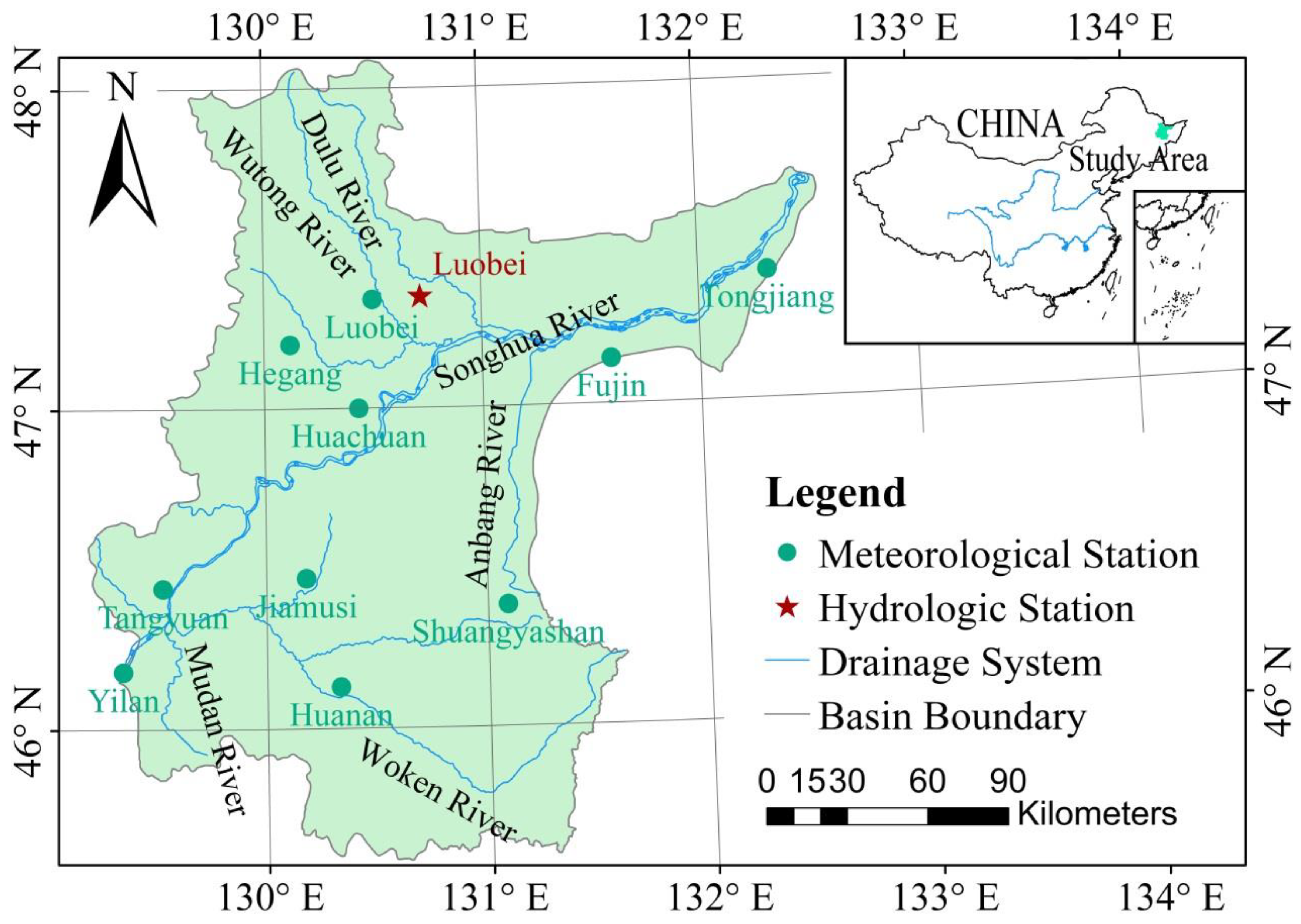
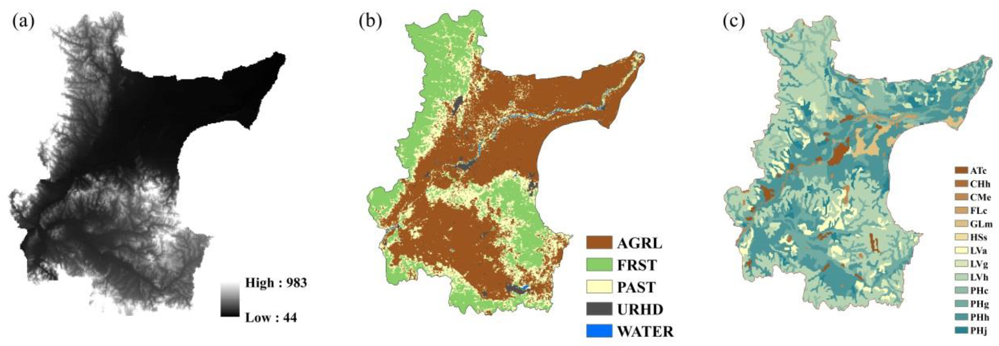
2.1. Study Area

This study used the coastal areas of Jiamusi city and Tongjiang city downstream of the Songhua River Basin as the research area. The area is located in the northeast of Heilongjiang Province and the hinterland of the Sanjiang Plain. The geographical position is 129°31′–132°29′ E and 46°22′–48°05′ N. The study area position is shown in Figure 1. The area of the main stream of the Songhua River below Jiamusi city is 13,365 km², the cultivated area is 692,670 ha and the ground elevation is generally between 60 m and 80 m. The region belongs to the mid-temperate continental monsoon climate, with four distinct seasons, a long winter and a short summer. The annual average temperature of the study area is 2.6 °C, the average annual wind speed is 3.8 m/s, and the annual average rainfall is 450 mm–650 mm. The Songhua River is a seasonally frozen river in the study area, and the freezing period is from late November to mid-April of the following year. The research area is rich in water and soil resources, with rapid development of agriculture, forestry, animal husbandry and fishery. The planting industry has become an important pillar of the national economy. It becomes the main grain-production bases in Heilongjiang and also the main commodity grain-producing areas in China [13]. Paddy fields are dominated by rice, while dry crops are dominated by corn and soybean. In this study area, the corn cultivar is Yinongyu 6 and the soybean cultivar is Dongnongdou 253. With the acceleration of social progress and economic development in the study area, the demand for water resources will continue to increase, especially in terms of agricultural irrigation, and this increase will result in the water resources carrying capacity of the region not fully meeting the requirements of social and national economic development. To solve this problem, this paper used the SWAT model as a tool to comprehensively formulate the optimal irrigation schedules for corn and soybean in the study area.

2.2. Research Methods

2.2.1. SWAT Model

SWAT is a physics-based, continuous distributed hydrological model that is used to predict the impact of management on water, sediment and agricultural material production in unmeasured watersheds. The main components include weather, water resource management and agricultural management. The main purpose of irrigation in the agricultural management module is to assess the impact of irrigation and crop growth on the irrigation system. The core of the module is to list the measures of land management and water management in the system. In this module, irrigation can be carried out according to a pre-set schedule. It can also trigger automatic irrigation by defining crop water stress or soil water stress thresholds in the model [14]. In order to improve the simulation accuracy, SWAT model is often used to subdivide a research basin into several sub-basins. Then, each sub-basin can be further divided into hydrological response units (HRU). An HRU refers to a combination of the same land-use type and soil type within the same sub-basin and is the smallest parcel unit in a sub-basin.

After the model is constructed, it needs to be further calibrated and verified. SWAT has a large number of hydrological parameters. Not all the parameters can significantly influence the model results. Therefore, the user must select the parameters that have greater effects on the study area to calibrate and reduce the cumulative error of the measured and simulated values, which can improve the accuracy of the model calculation. The parameters were determined by using the internal sensitivity analysis method Latin Hypercube (LH-OAT) [15] in SWAT-CUP. The optimal value of the parameters was determined by using each repetition of 1000 simulations of the SUFI-2 algorithm in the SWAT-CUP model. Afterwards, the runoff simulation process was verified using the observed monthly runoff data in the study area. The validation is based on the use of the model with calibrated parameters in an independent data mass so that the applicability of the model can be evaluated through several tests [16,17]. After the validation phases, if the model achieves a satisfactory performance, it becomes possible to perform model simulations according to different scenarios [18].

The model efficiency was evaluated by selecting the R², Nash-Sutcliffe (NS) and Percent Bias (PBIAS, %). R² measures the degree of correlation between the simulated value and the observed value, ranging from 0 to 1. R² = 1 indicates complete correlation, while R² = 0 indicates no correlation. NS can be used to evaluate the accuracy of model simulation, which intuitively reflects the fitting degree of the observed and simulated flow process. The closer NS is to 1, the higher the model efficiency is. When NS is negative, the model simulation value is not as good as the mean measured value [19]. PBIAS measures the average trend that the simulated data is larger or smaller than the observed. The optimal value of PBIAS is 0, and the low value indicates the accuracy of the model simulation. A positive value indicates that the deviation of the model estimation is small, and a negative value indicates that the model overestimates the deviation [20]. The calculation is shown in the following formulas. When all three indicators are consistent with the given criteria (R² > 0.7, NS > 0.5, PBIAS < ±25%), the model is considered suitable for simulation in the study area [20].

$$R^2={\left[{{\displaystyle \sum }}_{i=1}^n(Q_{obs,i}-{\overline{Q}}_{obs})\left(Q_{sim,i}-{\overline{Q}}_{sim}\right)\right]}^2/{{\displaystyle \sum }}_{i=1}^n{(Q_{obs,i}-{\overline{Q}}_{obs})}^2{{\displaystyle \sum }}_{i=1}^n{(Q_{sim,i}-{\overline{Q}}_{sim})}^2$$

(1)

$$NS=1-{{\displaystyle \sum }}_{i=1}^n{(Q_{obs}-Q_{sim})}^2/{{\displaystyle \sum }}_{i=1}^n{(Q_{obs}-{\overline{Q}}_{obs})}^2$$

(2)

$$PBIAS={{\displaystyle \sum }}_{i=1}^n(Q_{obs}-Q_{sim})/{{\displaystyle \sum }}_{i=1}^n{Q}_{obs}$$

(3)

where $Q_{obs}$ is the actual observed runoff, $Q_{sim}$ is the simulated runoff, ${\overline{Q}}_{obs}$ is the average of the actual observed runoff, ${\overline{Q}}_{sim}$ is the average of the simulated runoff, and i is the number of observation or simulation data.

2.2.2. Water Calculation

CropWat 8.0 [21] was used in this study to calculate reference crop evapotranspiration (ET₀) and effective precipitation (P_e). ET₀ is one of the main elements in the hydrological cycle, which is affected by the changes in air temperature, sunshine duration, and wind speed and so on [22]. P_e during the crop growth stages refers to the rainfall that can be supplied to the crop for evapotranspiration, thus reducing the demand for irrigation water [23]. For dry crops, P_e refers to the portion of the total rainfall that can be saved in the crop root layer to meet the needs of evapotranspiration, excluding surface runoff and leakage below the water-absorbing layer of the crop root system. The ET₀ in CropWat model was calculated using Penman formula, and the P_e was calculated using the recommended formula of the US Department of Agriculture Soil Conservation Bureau [24].

Crop water requirement (ET_c) refers to the sum of soil surface (or water surface) evaporation and plant transpiration under the conditions of suitable soil moisture and nutrients, adequate management, regular growth and high yield [25]. ET_c is affected by many factors, such as soil, crops, and climate. The methods for determining ET_c are mainly determined by field trials or theoretical calculations. In this study, a crop coefficients approach [26] was used to calculate ET_c. Crop coefficients [27] primarily depend on the dynamics of canopies, light absorption by the canopy, canopy roughness, which affects turbulence, crop physiology, leaf age and surface wetness. ET_c is calculated as follows.

$$E{T}_c=K_c\times E{T}_0$$

(4)

where ET_c is the daily crop water requirement (mm), K_c is the crop coefficient and ET₀ is the reference crop evapotranspiration (mm).

2.2.3. Coupling Degree between Effective Precipitation and Crop Water Requirement

The coupling degree between P_e and ET_c refers to the extent to which the effective precipitation meets the crop water requirements during the different growth stages, and its value is 0–1 [28]. The calculation formulas are as follows.

$$C_i=\{\begin{array}{c}1\\ P_{ei}/E{T}_{ci}\end{array} \begin{array}{c}{P}_{ei}\ge E{T}_{ci}\\ P_{ei}<E{T}_{ci}\end{array}$$

(5)

where i is the number of growth stages, C_i is the coupling degree, P_i is the effective precipitation (mm), and ET_ci is the crop water requirement (mm).

2.2.4. Sensitivity Index of Crop Water Production Function

The crop water production function refers to the functional relationship between crop yield and water consumption when the agricultural planting level is basically consistent [29,30], which provides a method for evaluating the multi-objective optimization of agricultural production, water productivity and profit maximization. Based on a large number of irrigation experiments, a series of crop water response models in different forms have been proposed by many domestic and international scholars. Common crop water production function models include the Jensen model, Blank model and Stewart model.

Based on previous studies, the Jensen function can better reflect the functional relationship between corn and soybean yield and water consumption [31,32]. Therefore, the Jensen function was used to analyze the crop water production function of corn and soybean in the downstream of the Songhua River Basin. The calculation formula is as follows.

$$\frac{Y}{Y_m}={{\displaystyle \prod }}_{i=1}^n{\left(\frac{E{T}_a}{E{T}_m}\right)}_i^{{\lambda }_i}$$

(6)

where i is the number of growth stages, λ_i is the sensitivity index for crop water deficit, n is the total number of growth stages, ET_a is the evapotranspiration during the growth stage under deficit irrigation (mm), ET_m is the maximum evapotranspiration during the growth stage under full irrigation (mm), Y is the crop yield under deficit irrigation (kg/hm²), and Y_m is the maximum crop yield under full irrigation (kg/hm²).

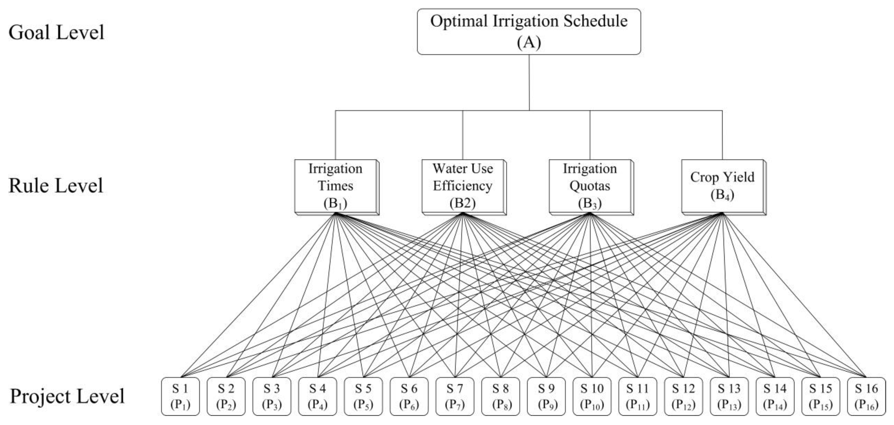
2.2.5. Optimal Assessment Method for Irrigation Schedule

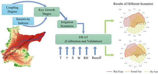
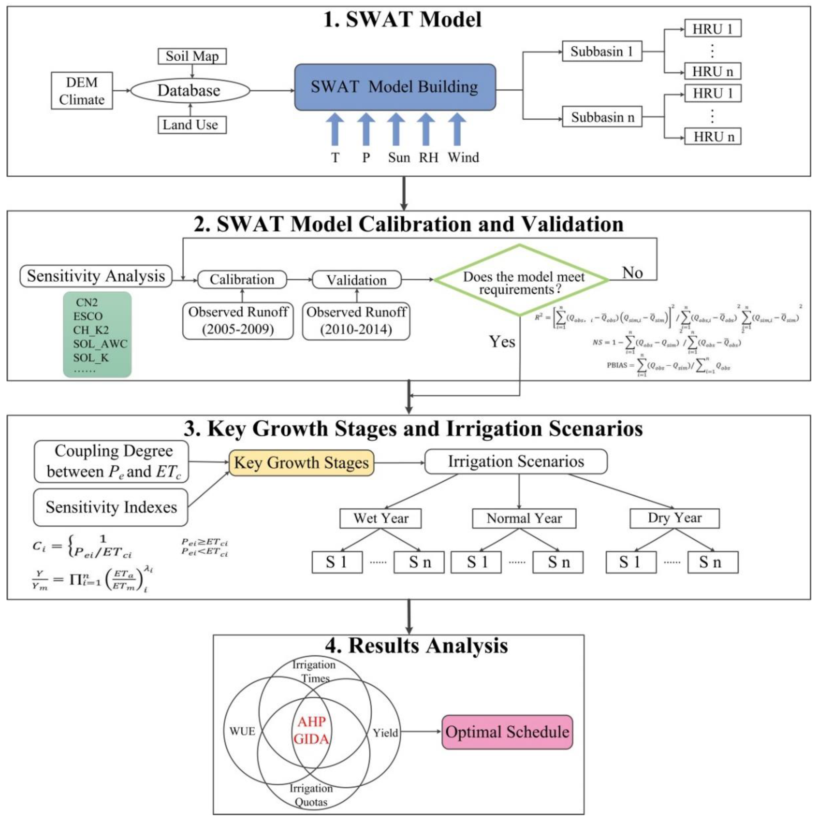
In this study, the AHP [33] was adopted to analyze the factors affecting the formulation of the irrigation schedule. The weight values determined by the AHP have many subjective factors [34], which makes the results unconvincing. Therefore, this paper combined GIDA [35] with the AHP to complement its advantages and obtain more reasonable and scientific evaluation results. The factors selected to influence irrigation schedule included irrigation times, WUE, irrigation quotas, crop yield. Crop yield were taken from the calibrated SWAT model. WUE is defined as grain yield divided by the evapotranspiration (ET_a) during the growing season [36]. The calculation formula of WUE is as follows.

$$\mathrm{WUE}=Y/E{T}_a$$

(7)

where Y is the crop yield (kg/hm²), and ET_a is the evapotranspiration during the growth stage (mm).

2.3. Research Ideas

Based on the above analysis, the technical process of this paper is shown in Figure 2. First, based on DEM, land use, soil and climatic conditions (temperature (T), rainfall (P), sunshine (Sun), relative humidity (RH) and Wind speed (Wind)), the SWAT model of the study area was constructed and was divided into sub-basins and HRUs. Second, the model was calibrated and verified. Third, the key growth stages of crops were determined, and different irrigation scenarios were set. Fourth, the simulation results were analyzed based on the AHP–GIDA to obtain optimal irrigation schedules.

2.4 Data Sources

This study required terrain, land-use, soil and hydro-meteorological data. The topographic data for the study area included a digital elevation model (DEM) with a resolution of 30 m that was downloaded from the Chinese Academy of Sciences’ Geospatial Data Cloud. The downloaded DEM was spliced and clipped in ArcGIS. The land-use classification system adopted by the SWAT model is the land-use classification system of the US Geological Survey (USGS), so the land-use types in the basin were code-transformed by establishing index tables. The land-use reclassification is shown in Figure 3. The land-use types in the basin are divided into five categories, namely, AGRL, FRST, PAST, URHD, and WATER. The AGRL and FRST are two major types of land use. Soil data from the Harmonized World Soil Database (HWSD), which was constructed by the United Nations Food and Agriculture Organization (FAO) and the Vienna International Institute for Applied Systems Analysis (IIASA), use the soil moisture signature software SPAW (soil, plant, atmosphere, and water) from Washington State University, which was converted to USGS soil parameters and imported into the model database. Li [19] established a soil database using SPAW software, so as to establish a SWAT model to study water cycle and water resources in Songhua River Basin under the changing environment. The results show that SPAW software was suitable for the calculation of soil moisture data in the Songhua River Basin. Thirteen soil types were extracted from the downstream region of the Songhua River Basin. The spatial distribution of the soil types is shown in Figure 3. Meteorological data were obtained from the National Meteorological Science Data Sharing Service Platform, including the daily maximum temperature, minimum temperature, sunshine hours, average wind speed, average relative humidity and precipitation. The monthly runoff at the hydrological station was obtained from the Heilongjiang Water Conservancy and Hydropower Investigation and Design Institute. Ten meteorological stations (Tangyuan, Yilan, Huanan, Shuangyashan, Jiamusi, Luobei, Huachuan, Hegang, Fujin and Tongjiang) and the Luobei Hydrological Station were selected from the basin.

This study assumed that the crop coefficient (Kc) is the same value every year. The crop growth stages and Kc are referred to in

Table 1. Crop coefficient and development stages.

Crops	Development Stages					Sowing (mm/dd)	Harvesting (mm/dd)	Total (Days)
		Initial	Development	Middle	Late
Corn	Growth stages	Establishment	Vegetative	Reproductive	Maturity	5/9	9/28	143
	Date (mm/dd)	5/9–6/15	6/16–7/28	7/29–8/29	8/30–9/28
	KC	0.30	-	1.10	0.35
Soybean	Growth stages	Establishment	Pod formation	Seed enlargement	Maturity	5/1	9/28	151
	Date (mm/dd)	5/1–6/19	6/20–7/24	7/25–9/2	9/3–9/28
	KC	0.32	-	0.96	0.32

. The crop data were obtained from the Heilongjiang Statistical Yearbook. As shown in Table 1, both the development of corn and soybean were divided into four stages.

3. Results and Discussion

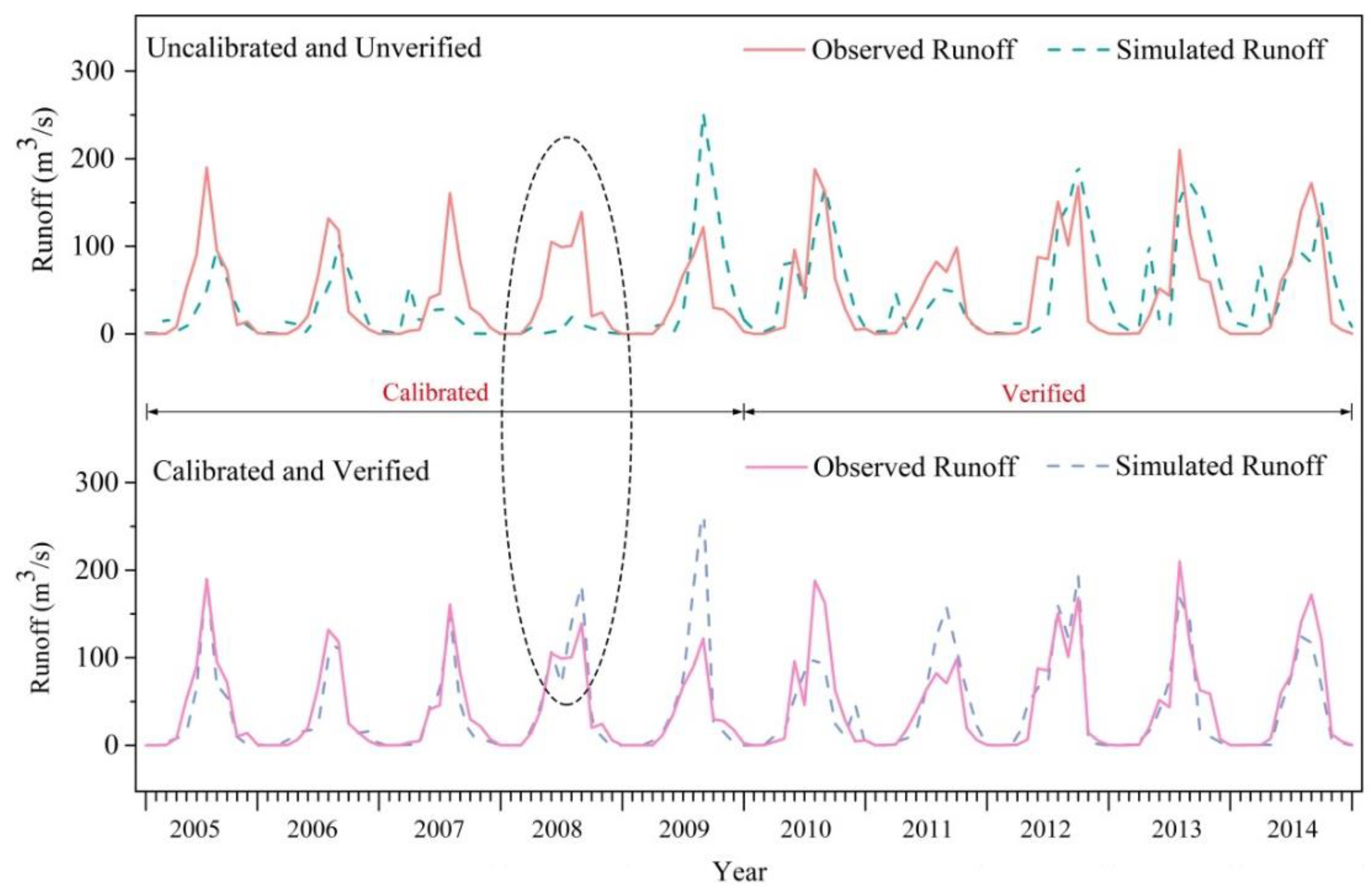
3.1. Performance Evaluation of the SWAT Model

Considering the characteristics of the study area and referring to previous studies on parameter selection and sensitivity analysis of the SWAT model [37], this paper adopted the observed monthly runoff data of Luobei Hydrological Station from 2005 to 2009 to calibrate the runoff simulation process, in which the selected sensitive parameters were CN2, ESCO, CH_K2, SOL_AWC, SOL_K, ALPHA_BF, GW_DELAY, GWQMN, REVAPMN, and GW_REVAP. Then, the runoff simulation process was verified using the observed monthly runoff data of Luobei Station from 2010 to 2014. For the calibration period, the R², NS and PBIAS were 0.79, 0.67 and −1.87%, respectively. For the validation period, the R², NS and PBIAS were 0.76, 0.75 and 7.3%, respectively. All three indicators were consistent with the given criteria.

Figure 4 shows the results of a comparison between the observed and simulated runoff for the calibration (2005–2009) and validation (2010–2014) periods. The peak times of observed and simulated runoff during the calibration period and validation period were the same, and the recession periods were also consistent. Among these times, the calibration period was best in 2006 and 2007 and was slightly worse in 2005, 2008 and 2009. The verification period was best in 2012 and 2013, and the simulation effect was slightly worse in 2010, 2011 and 2014. Generally, the SWAT model was suitable for application to this study area.

3.2. Key Growth Stages

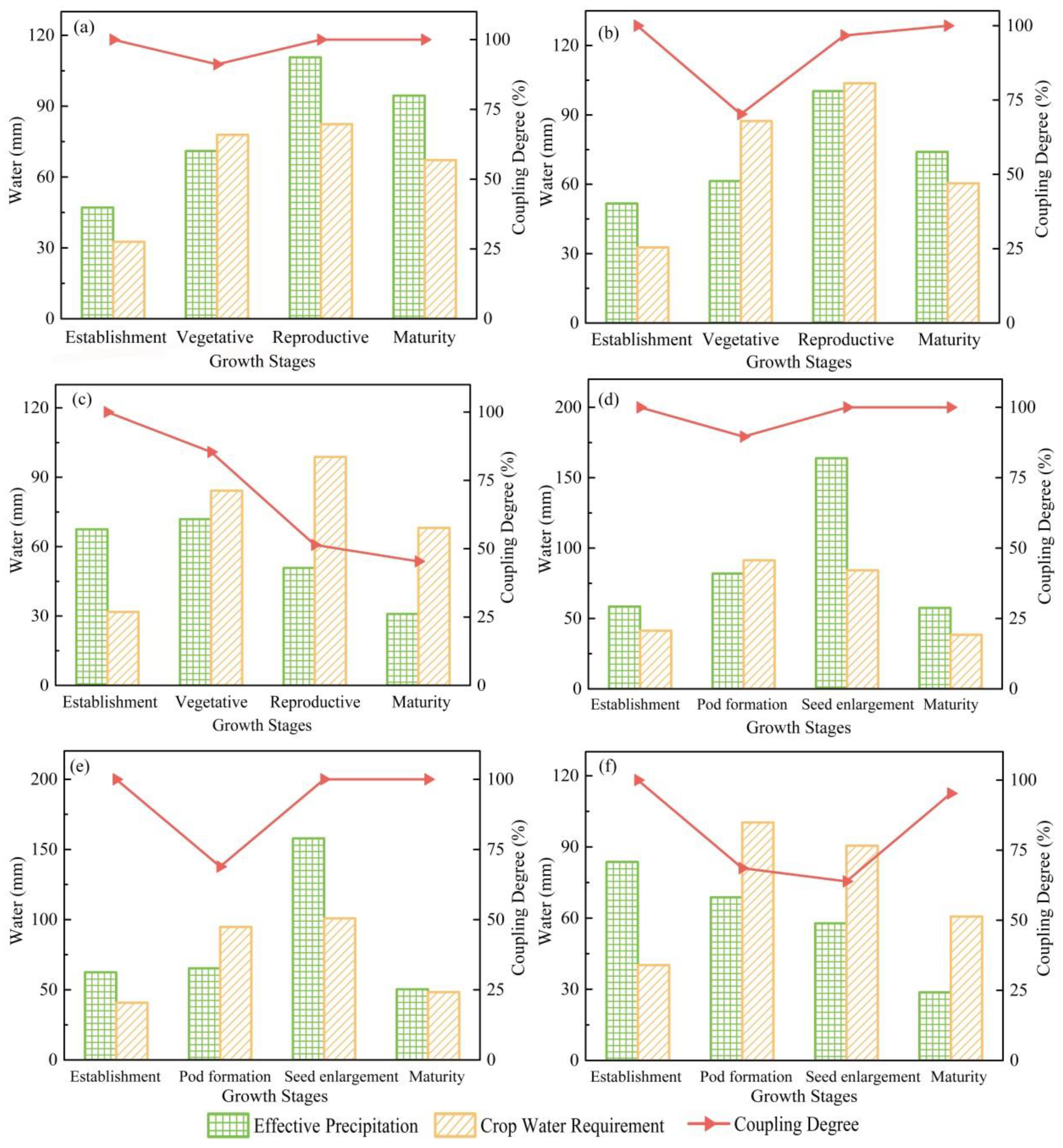
3.2.1. Calculation of the Coupling Degree between P_e and ET_c

According to many years of precipitation data from the meteorological stations in the study area, three typical years were determined by the P III frequency curve: wet year (precipitation frequency is 25%), normal year (precipitation frequency is 50%) and dry year (precipitation frequency is 85%).

The P_e, ET_c and the coupling degree under different typical years are shown in Figure 5. The P_e generally increased first and then decreased. The coupling degree between P_e and ET_c was first reduced and then increased.

It can be seen from Figure 5 that there was more P_e during the vegetative and reproductive stages of corn and less P_e during the establishment stage. There was abundant rainfall in the wet year, and P_e was the largest. The coupling degrees between P_e and ET_c in the corn growth stages of the wet year and the normal year were close to 100%, except for the vegetative stage, indicating that the precipitation basically met the requirement of corn growth and could provide water for the latter stages. The water shortage was most serious in the middle and late stages of the dry year. The coupling degree between P_e and ET_c was lower in pod formation and seed enlargement stage, and higher in establishment and maturity stage. Similar to corn, the precipitation in the wet year basically met the demand for water and water shortage was serious in middle and late period of soybean in the normal and dry year.

3.2.2. Calculation of Sensitivity Indexes of Crop Water Production Function

In this paper, the sensitivity indexes were determined by setting different irrigation treatments in the growth stages, which were used to construct the crop water production function [38,39]. To construct the relative treatments of Y/Y_m and ET_ai/ET_mi, an adequate irrigation treatment,namely, CK,was assumed (crops were not affected by water stress), and irrigation water was the same at each growth stage. Then, 14 deficit irrigation treatments were set up by arranging and combining, and a single irrigation water event was consistent with CK. Treatments 1–14 were inadequate irrigation and the irrigation quota at each growth stage was 40 mm, which can be seen from

Table 2. Crop water production function irrigation treatments.

Treatments	Irrigation Water of Corn Growth Stages/mm				Irrigation Water of Soybean Growth Stages/mm
	Establishment	Vegetative	Reproductive	Maturity	Establishment	Pod Formation	Seed Enlargement	Maturity
CK	40	40	40	40	40	40	40	40
1	40	40	40	0	40	40	40	0
2	40	40	0	40	40	40	0	40
3	40	0	40	40	40	0	40	40
4	0	40	40	40	0	40	40	40
5	40	40	0	0	40	40	0	0
6	40	0	40	0	40	0	40	0
7	40	0	0	40	40	0	0	40
8	0	40	40	0	0	40	40	0
9	0	40	0	40	0	40	0	40
10	0	0	40	40	0	0	40	40
11	40	0	0	0	40	0	0	0
12	0	40	0	0	0	40	0	0
13	0	0	40	0	0	0	40	0
14	0	0	0	40	0	0	0	40

.

The irrigation treatments in Table 2 were separately input into the SWAT model according to the set irrigation mode as agricultural management measures, and the yield as well as the evapotranspiration were simulated for the growth stages from 1985 to 2014. The sensitivity indexes of Jensen were calculated by the nonlinear regression analysis module of the SPSS software. The results are shown in

Table 3. Sensitivity indexes of water production function.

Sub-Basin Number	Corn Growth Stages				Soybean Growth Stages
	Establishment	Vegetative	Reproductive	Maturity	Establishment	Pod Formation	Seed Enlargement	Maturity
5	0.04	0.04	0.32	0.26	0.17	0.36	0.49	0.28
6	0.03	0.34	0.42	0.34	0.21	0.42	0.40	0.26
7	0.05	0.05	0.39	0.13	0.20	0.38	0.42	0.27
8	0.03	0.35	0.43	0.06	0.10	0.45	0.45	0.28
9	0.02	0.11	0.30	0.02	0.19	0.36	0.42	0.27
10	0.03	0.14	0.47	0.20	0.18	0.38	0.45	0.23
11	0.05	0.31	0.47	0.18	0.25	0.35	0.55	0.25
12	0.05	0.29	0.46	0.01	0.24	0.36	0.52	0.27
13	0.01	0.23	0.32	0.06	0.20	0.41	0.51	0.24
14	0.01	0.23	0.50	0.32	0.24	0.42	0.45	0.26
15	0.04	0.18	0.39	0.15	0.10	0.32	0.56	0.23
16	0.05	0.30	0.34	0.29	0.23	0.45	0.46	0.28
17	0.05	0.18	0.44	0.09	0.17	0.37	0.38	0.23
18	0.04	0.13	0.36	0.08	0.12	0.32	0.55	0.25
19	0.03	0.36	0.32	0.14	0.23	0.44	0.39	0.26
20	0.04	0.14	0.48	0.26	0.21	0.39	0.40	0.27
21	0.02	0.09	0.45	0.10	0.15	0.39	0.48	0.24
22	0.03	0.01	0.41	0.06	0.22	0.38	0.56	0.23
23	0.05	0.05	0.41	0.27	0.12	0.41	0.55	0.28
24	0.01	0.33	0.42	0.35	0.25	0.32	0.37	0.27
25	0.03	0.31	0.47	0.11	0.13	0.40	0.41	0.28
26	0.02	0.32	0.48	0.17	0.13	0.35	0.46	0.26
27	0.01	0.35	0.44	0.19	0.10	0.36	0.53	0.26
28	0.05	0.41	0.43	0.06	0.24	0.38	0.57	0.23
29	0.02	0.20	0.42	0.11	0.24	0.43	0.45	0.24
30	0.01	0.26	0.48	0.28	0.19	0.37	0.42	0.26
31	0.05	0.05	0.31	0.33	0.14	0.34	0.57	0.23
Average	0.03	0.21	0.41	0.17	0.18	0.38	0.47	0.26

Note: There were no land-use types suitable for intensive cultivation in sub-basins 1–4, so corn and soybean were not planted in these four sub-basins.

.

Table 3 shows the water sensitivity indexes of corn and soybean at different growth stages on the sub-basin scale of the study area, as calculated by the Jensen model. The regional average water sensitivity index of the corn establishment stage was 0.03, which was the smallest of all growth stages. The average values at vegetative, reproductive and maturity were 0.21, 0.41 and 0.17, respectively. The values of soybean at pod formation and seed enlargement were higher, but the values at establishment and maturity were relatively lower.

3.2.3. Determination of Key Growth Stages

Vegetative and reproductive of corn and pod formation and seed enlargement of soybean were considered the key growth stages based on the analysis of the coupling degree between P_e and ET_c and the sensitivity indexes of the crop water production function. Sun et al. [40] showed that water stress at different growth stages of corn will have adverse effects on plants, especially in vegetative and reproductive. Han et al. [41] also showed that pod formation and seed enlargement of soybean have higher water requirements. This result is consistent with the research results of this paper.

3.3. Setting of Irrigation Scenarios

In this paper, 16 irrigation scenarios with different irrigation quotas and irrigation times were set for crops in the same typical year. The setting principles were as follows: ① Scenario 1 was the basic irrigation schedule simulated by the SWAT automatic irrigation module. ② Scenarios 2–16 were irrigated only in key growth stages. ③ The irrigation quotas in Scenarios 2, 5, 8, 11 and 14 were 1, 1/3, 2/3, 4/3 and 5/3 times, respectively, of the quotas in the key growth stages of Scenario 1. These scenarios were irrigated only once in each growth stage. ④ The total irrigation quota in Scenarios 3 and 4 were equal to that in Scenario 2. Furthermore, the irrigated times in each growth period were 2 and 3 times, respectively, and the irrigation quotas in each growth stage was the arithmetic average of Scenario 2. Scenarios 6, 7, 9, 10, 12, 13, 15, and 16 were set by the same standards. The specific irrigation scenarios are shown in Figure 6. Taking Figure 6a as an example, the scenario with the same column color indicated that the total irrigation quota was the same during entire development stage. The number of columns in the same irrigation scenario represented the irrigation times, and the column height indicated the irrigation quota of the crop at each growth stage.

3.4. Optimal Irrigation Schedule

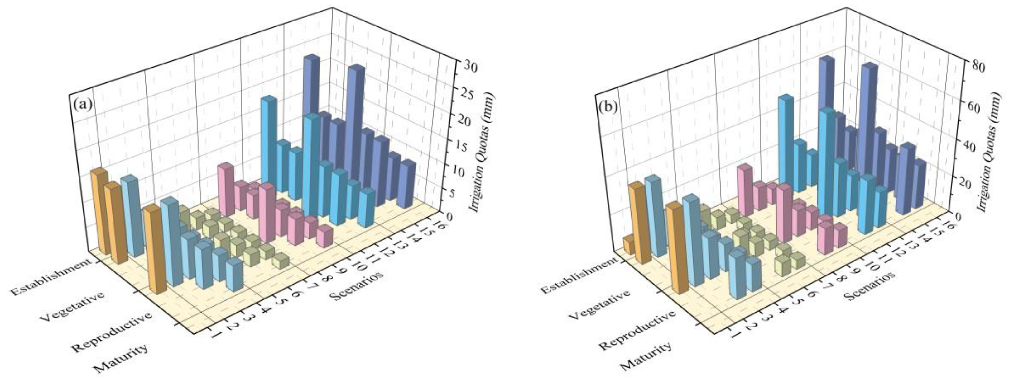
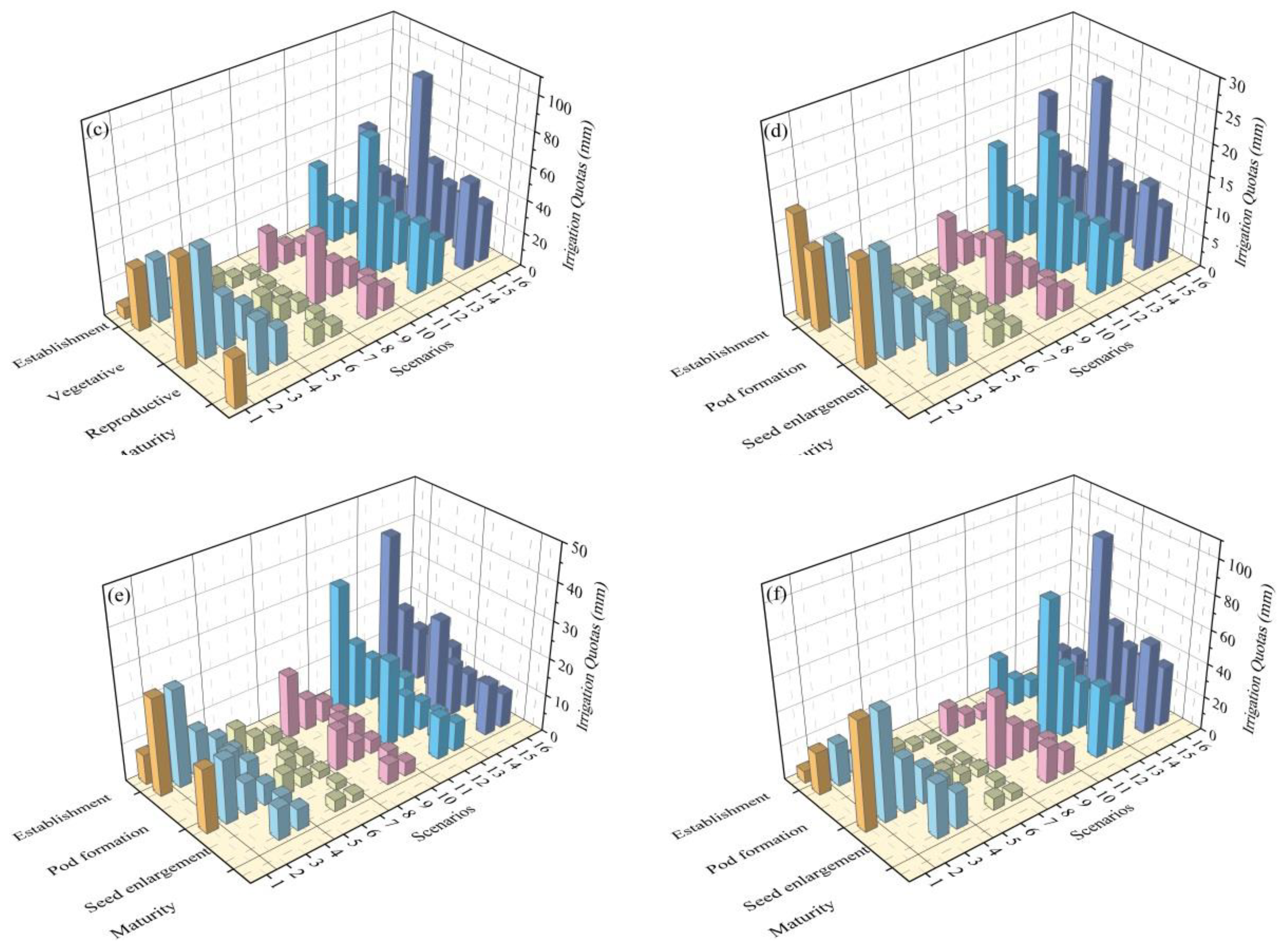
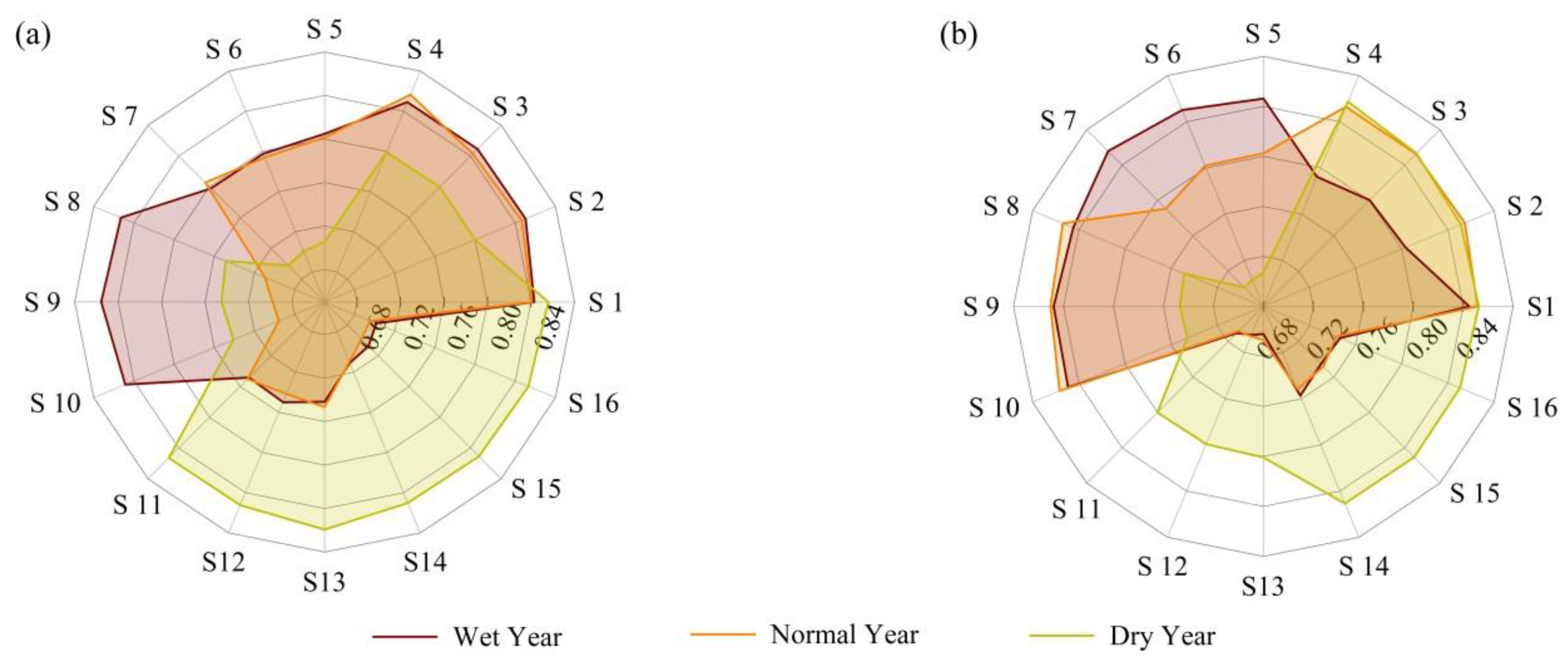
3.4.1. Analysis of Irrigation Scenario Results

According to the standard of the local water quotas in Heilongjiang Province (DB23/T 727-2017), the study area is located in the Sanjiang Plain Irrigation Division of Heilongjiang Province [42]. The irrigation quotas for corn and soybean in this area are shown in

Table 4. Crop irrigation quotas standards.

Crop	Typical Years	Irrigation Quotas (mm)
		Standards	Water Balance Method
Corn	Wet Year	27.0	58.0
	Normal Year	59.4–86.4	102.0
	Dry Year	86.4–113.4	120.0
Soybean	Wet Year	27.0	50.0
	Normal Year	55.8–84.6	93.0
	Dry Year	84.6–112.5	103.0

. In addition, Table 4 includes irrigation quotas of corn and soybean in different typical years calculated by using the water balance method in Irrigation and Drainage Engineering [43].

As shown in Table 4, the standard irrigation quotas for both corn and soybean were 27.0 mm in the wet year. The irrigation quotas simulated by SWAT model were both 47.0 mm, which were slightly higher than the standard. But the corresponding values turned to 58.0 mm and 50.0 mm when water balance method was used. Therefore, SWAT simulation accuracy was higher in the wet year. According to the water balance method, in the normal year, the irrigation quota was 102.0 mm for corn and 93.0 mm for soybean, while simulated by SWAT model the corn quota was 91.0 mm and soybean quota was 51.0 mm, which were closer to the standard. In the dry year, the simulated quota of corn was 136.0 mm, slightly higher than the standard and the soybean irrigation quota was 96.0mm, which was within the standard range. In general, the irrigation quotas simulated by SWAT were closer to the standard than those calculated by the water balance method and the data were slightly higher than the standard, which may be affected by the selection of typical years. As a result, SWAT model was suitable for the simulation of irrigation schedule in this region. Figure 7 shows the irrigation quotas, irrigation times, yield and WUE of crops under different irrigation scenarios. The sizes of the points in the figure indicate the different irrigation times.

As shown in Figure 7, generally speaking, as the irrigation quota increased, the crop yield increased. However, as the irrigation quota increased, the rate of increase in production decreased, which may result in crop yield loss. This result is consistent with the conclusion drawn by Lu et al. [44]. For yield and WUE, the peaks did not necessarily coincide. Although the yield of soybean in Scenario 3 in the dry year was lower than that in Scenario 4, the WUE presented a rising state. In addition, for the same irrigation quota, the crop yield and WUE also varied to different degrees due to different irrigation times. The irrigation quotas of corn in Scenarios 5, 6 and 7 in the normal year were the same. The yield of Scenario 6 was 146 kg/m² less than that of Scenario 5, but that of Scenario 7 was 23 kg/m² higher than that of Scenario 6. Due to meteorological factors such as precipitation, there were significant differences in the changes in yield and WUE in the same scenario in different typical years. The three typical years were all irrigated 4 times in Scenario 3. The yield of soybean in the normal year increased by 44 kg/m² compared with that in the wet year, but the WUE decreased by 3.4%. Therefore, the results of the irrigation schedule in different scenarios were different, and it was difficult to directly judge the optimal irrigation scenario. It was necessary to combine all the influencing factors for judgment.

3.4.2. Determination of Optimal Irrigation Schedule

According to the interrelationship and membership among the indexes affecting the irrigation schedule [45], a comprehensive evaluation model of three levels was established by the AHP. The diagram of the hierarchical structure is shown in Figure 8. The first layer was the target layer, which was the optimal irrigation schedule. The second layer was the criterion layer, including irrigation times B₁, WUE B₂, irrigation quotas B₃ and crop yield B₄. The third layer was the scheme layer, including 16 different irrigation scenarios. The target layer was composed of one element, while the criterion layer and the scheme layer were composed of multiple elements. Each element of the same layer had different influences on the upper layer.

Based on the 1–9 scale method of the AHP and the importance of each evaluation index on the irrigation schedule, the judgment matrixes of the lower-level index relative to the upper-level index were calculated. The weights of each index were calculated, and a consistency test was run [46]; the results met the requirements. According to the results of the AHP, the characteristic matrix of weights were constructed to calculate the gray relational degree [47], and then the optimal irrigation schedule of crops were obtained. The absolute correlation degree are shown in Figure 9.

It can be seen from Figure 9 that under different irrigation scenarios, the advantages and disadvantages of irrigation schedules were significantly different. In the process of crop growth, more irrigation water may not be the best effect. The scenario of irrigation in the key growth stages was better than that in the whole period. A moderate deficit was more conducive to increasing the crop yield and WUE, which was consistent with the study by Candogan and Yazgan [48]. Payero et al. [49] believed that water consumption decreased with decreasing irrigation. A certain range of water stress can significantly improve the WUE of corn. Under the same irrigation quota, more irrigation times will lead to an increase in crop yield and WUE. However, with the increase in irrigation times, the irrigation schedule may not perform optimally, and the WUE may show a downward trend. One of the important reasons for this change is that with increasing irrigation times, the water consumption of soil evaporation increases [50]. In addition, more irrigation times will bring cause several inconveniences in terms of production and life.

According to the principle of correlation analysis, as the correlation degree increases, the closer the value is to the optimal irrigation schedule. The optimal irrigation schedules of corn and soybean in different typical years are shown in

Table 5. Crop optimal irrigation schedule.

Crops	Typical Years	Optimal Schedule	Irrigation Water of the Development Stages (mm)								Irrigation Quotas (mm)	Irrigation Times (Times)
			Initial	Development			Middle			Late
Corn	Wet Year	S9		5.0		5.0	5.5		5.5		21	4
	Normal Year	S4		13.3	13.3	13.3	14.7	14.7	14.7		84	6
	Dry Year	S13		16.7	16.7	16.7	28.0	28.0	28.0		134	6
Soybean	Wet Year	S7		1.3	1.3	1.3	2.0	2.0	2.0		10	6
	Normal Year	S10		5.7	5.7	5.7	3.7	3.7	3.7		28	6
	Dry Year	S4		8.3	8.3	8.3	21.3	21.3	21.3		89	6

.

Table 5 shows that in the years with less rainfall, the irrigation quotas and times must be increased to meet the water requirements of crops. Due to high precipitation in the wet year, corn can only be satisfied by applying irrigation twice in each key growth stage. In the normal year and dry year, it is necessary to irrigate six times throughout all key growth stages to ensure the growth of crops. The soybeans of the three typical years required six irrigation times in the entire key growth stage, with an irrigation quota of 10 mm in the wet year, 28 mm in the normal year and up to 89 mm in the dry year.

4. Conclusions

In this study, the SWAT model was constructed to simulate crop irrigation schedules in downstream regions of the Songhua River Basin. The irrigation requirement rules and the optimal irrigation schedule of corn and soybean were defined for different typical years. The main conclusions are as follows:

(1) The SWAT model was established for the study area, and the monthly runoff of the basin was calibrated to improve the simulation accuracy. The evaluation indexes R², NS, PBIAS were 0.79, 0.67 and −1.87%, respectively, in the calibration period and 0.76, 0.75, and 7.3%, respectively, in the verification period, which met the accuracy requirements. The results showed that the performance of the SWAT model was stable and suitable for the simulation of the study area.

(2) Determining the key growth stages by analyzing the coupling degree between P_e and ET_c and the sensitivity indexes. The analysis was carried out from multiple angles to avoid the inaccuracies caused by using a single factor. Vegetative and reproductive of corn and pod formation and seed enlargement of soybean were considered the key growth stages.

(3) The comprehensive analysis of different optimization scenarios for two crops in different typical years showed that deficit treatments during the growth stages were beneficial to improving crop yield and WUE. Suitable irrigation quotas and times can save water resources and reduce the risk of yield reductions. The optimal treatment of corn in the wet year is Scenario 9, which includes applying irrigation 4 times throughout the entire key growth stages. The best irrigation method for the normal year was to irrigate 6 times at vegetative and reproductive for a total of 84 mm. Scenario 13 performed optimally and was irrigated 6 times in the entire key growth stage in a dry year, with 134 mm. Soybean was irrigated 6 times in the entire key growth stage, and the irrigation quota was 10 mm in the wet year. The useful irrigation quota of a normal year was 28 mm, with 6 irrigation times in the pod formation and seed enlargement stages. The water used in the dry year was much higher than that used in two typical years, at 89 mm. Water needed to be applied 6 times in the key growth stages.

(4) This method for identifying crop irrigation schedules had better results in different non-sufficient irrigation schedules of corn and soybean, which was in accordance with objective reality, and the results provided a reliable scientific basis for decision-making in this field and a new evaluation idea of strong practicality.

In general, the optimal irrigation schedule selected in this paper can effectively save irrigation water and improve WUE under the condition of ensuring a stable crop yield, which is of great significance for guiding agricultural production. However, the irrigation scenarios set for corn and soybean in this paper are not comprehensive enough to fully reflect the irrigation combination in the study area, which needs to be further improved in the next step.

References

1. Singh, A. An overview of the optimization modelling applications. J. Hydrol. 2012, 466, 167–182. [Google Scholar] [CrossRef]
2. Wang, Y.B.; Liu, D.; Cao, X.C.; Yang, Z.Y.; Song, J.F.; Chen, D.Y.; Sun, S.K. Agricultural water rights trading and virtual water export compensation coupling model: A case study of an irrigation district in China. Agric. Water Manag. 2017, 180, 99–106. [Google Scholar] [CrossRef]
3. Liu, D.; Qi, X.C.; Fu, Q.; Zhu, W.F.; Zhang, L.L.; Muhammad, A.F.; Muhammad, I.K.; Li, T.X.; Cui, S. A resilience evaluation method for a combined regional agricultural water and soil resource system based on Weighted Mahalanobis distance and a Gray-TOPSIS model. J. Clean. Prod. 2019, 229, 667–679. [Google Scholar] [CrossRef]
4. Li, M.; Fu, Q.; Singh, V.P. An optimal modeling approach for managing agricultural water-energy-food nexus under uncertainty. Sci. Total Environ. 2019, 651, 1416–1434. [Google Scholar] [CrossRef]
5. Wang, Y.L.; He, L.Y. Review and application of crop growth simulation models. J. Huazhong Agric. Univ. 2005, 24, 529–535. [Google Scholar]
6. Chi, H.; Bai, Y.; Wang, H.T.; Zhao, J. Application of HYDRUS-3D in simulation of soil water infiltration process. J. Comput. Appl. Chem. 2014, 31, 531–535. [Google Scholar]
7. Asgharzadeh, M.A.; Heidarpour, M.; Shayannejad, M.; Rasti-Barzoki, M. Development of hadis algorithm for deficit irrigation scheduling. Irrig. Drain. 2018, 67, 345–353. [Google Scholar] [CrossRef]
8. Geerts, S.; Raes, D.; Garcia, M. Using aquacrop to derive deficit irrigation schedules. Agrict. Water Manag. 2010, 98, 213–216. [Google Scholar] [CrossRef]
9. Attia, A.; Rajan, N.; Xue, Q.W.; Nair, S.; Ibrahim, A.; Hays, D. Application of dssat-ceres-wheat model to simulate winter wheat response to irrigation management in the Texas high plains. Agrict. Water Manag. 2016, 165, 50–60. [Google Scholar] [CrossRef]
10. Gosain, A.K.; Rao, S.; Srinivasan, R.; Reddy, N.G. Return-flow assessment for irrigation command in the palleru river basin using swat model. Hydrol. Process. 2005, 19, 673–682. [Google Scholar] [CrossRef]
11. Chen, Y.; Marek, G.W.; Marek, T.H.; Brauer, D.K.; Srinivasan, R. Assessing the efficacy of the SWAT auto-irrigation function to simulate irrigation, evapotranspiration and crop response to management strategies of the Texas high plains. Water 2017, 9, 509. [Google Scholar] [CrossRef]
12. Cui, Y.L.; Wu, D.; Wang, S.W.; Wen, J.H.; Wang, H.L. Simulation analysis of irrigation water consumption in southern multi-source irrigation district based on improved SWAT model. Trans. Chin. Soc. Agric. Eng. 2018, 341, 102–108. [Google Scholar]
13. Zhang, L.L.; Li, H.; Liu, D.; Fu, Q.; Li, M.; Muhammad, A.F.; Muhammad, I.K.; Li, T.X. Identification and application of the most suitable entropy model for precipitation complexity measurement. Atmos. Res. 2019, 221, 88–97. [Google Scholar] [CrossRef]
14. Uniyal, B.; Dietrich, J.; Vu, N.Q.; Jha, M.K.; Arumi, J.L. Simulation of regional irrigation requirement with SWAT in different agro-climatic zones driven by observed climate and two reanalysis datasets. Sci. Total Environ. 2019, 649, 846–865. [Google Scholar] [CrossRef]
15. Abbaspour, K.C.; Yang, J.; Maximov, I.; Siber, R.; Bogner, K.; Mieleitner, J.; Zobrist, J.; Srinivasan, R. Modelling hydrology and water quality in the pre-alpine/alpine thur watershed using swat. J. Hydrol. 2007, 333, 413–430. [Google Scholar] [CrossRef]
16. Pereira, D.R.; Martinez, M.A.; Almeida, A.Q.; Pruski, F.F.; Silva, D.D.; Zonta, J.H. Hydrological simulation using SWAT model in headwater basin in southeast Brazil. Eng. Agríc. 2014, 34, 789–799. [Google Scholar] [CrossRef]
17. Jha, M. SWAT: Model use, calibration, and validation. Trans. Asabe 2012, 55, 1345–1352. [Google Scholar]
18. Marek, G.W.; Gowda, P.H.; Evett, S.R.; Baumhardt, L.; Brauer, D.K.; Howell, T.A.; Marek, T.H.; Srinivasan, R. Calibration and validation of SWAT model for predicting daily ET over irrigated crops in Texas high plains using lysimetric data. Trans. Asabe 2017, 59, 611–622. [Google Scholar]
19. Li, F.P.; Zhang, G.X.; Xu, J. Spatiotemporal variability of climate and streamflow in the Songhua River Basin, northeast China. J. Hydrol. 2014, 514, 53–64. [Google Scholar] [CrossRef]
20. Moriasi, D.N.; Arnold, J.G.; Liew, M.W.V.; Bingner, R.L.; Harmel, R.D.; Veith, T.L. Model evaluation guidelines for systematic quantification of accuracy in watershed simulations. Trans. Asabe 2007, 50, 885–900. [Google Scholar] [CrossRef]
21. Allen, R.G.; Pereira, L.S.; Raes, D.; Smith, M. Crop Evapotranspiration for Computing Crop Water Requirement. In Irrigation and Drainage Paper 56; FAO: Rome, Italy, 1998. [Google Scholar]
22. Dinpashoh, Y.; Jhajharia, D.; Fakheri-Fard, A.; Singh, V.P.; Kahya, E. Trends in reference crop evapotranspiration over Iran. J. Hydrol. 2011, 399, 422–433. [Google Scholar] [CrossRef]
23. Liu, Y.; Wang, L.; Ni, G.H.; Cong, Z.T. Spatial distribution characteristics of irrigation water requirement for main crops in china. Trans. Chin. Soc. Agrict. Eng. 2009, 25, 6–12. [Google Scholar]
24. Todorovic, M. Crop Evapotranspiration. Water Encycl. 2005, 3, 571–579. [Google Scholar]
25. Pan, Y.Q.; Cai, H.C. Comparison of crop water requirements computed by single crop coefficient approach and dual crop coefficient approach. J. Hydraul. Eng. 2002, 3, 50–54. [Google Scholar]
26. Justice, C.; Townshend, J. Special issue on the moderate resolution imaging spectroradiometer (modis): A new generation of land surface monitoring. Remote Sens. Environ. 2002, 83, 1–2. [Google Scholar] [CrossRef]
27. Guo, J.L.; Yin, G.H.; Gu, J.; Liu, Z.X. Determination of irrigation scheduling of spring maize in different hydrological years in Fuxin Liaoning Province based on CROPWAT model. Chin. J. Ecol. 2016, 35, 3428–3434. [Google Scholar]
28. Zhang, Q.P.; Yang, X.G.; Xue, C.Y.; Yan, W.X.; Yang, J.; Zhang, T.Y.; Bauman, B.A.M.; Wang, H.Q. Coupling analysis of water requirement and precipitation of upland rice crops in Beijing. Trans. Chin. Soc. Agrict. Eng. 2007, 23, 51–56. [Google Scholar]
29. Kozlowski, T.T. Water Deficits and Plant Growth; Water Relation Plants; Elsevier: Amsterdam, The Netherlands, 1983; pp. 342–389. [Google Scholar]
30. Oweis, T.; Hachum, A. Optimizing supplemental irrigation: Tradeoffs between profitability and sustainability. Agrict. Water Manag. 2009, 96, 511–516. [Google Scholar] [CrossRef]
31. Ferreira, D.B.; Rao, V.B. Recent climate variability and its impacts on soybean yields in southern brazil. Theor. Appl. Climatol. 2011, 105, 83–97. [Google Scholar] [CrossRef]
32. El-Hendawy, S.E.; Schmidhalter, U. Optimal coupling combinations between irrigation frequency and rate for drip-irrigated maize grown on sandy soil. Agric. Water Manag. 2010, 97, 439–448. [Google Scholar] [CrossRef]
33. Fu, Q. Data Processing Methods and their Agricultural Applications; Science Press: Beijing, China, 2006; pp. 483–491. [Google Scholar]
34. Macharis, C.; Springael, J.; Brucker, K.D.; Verbeke, A. Promethee and AHP: The design of operational synergies in multicriteria analysis: Strengthening Promethee with ideas of AHP. Eur. J. Oper. Res. 2004, 153, 307–317. [Google Scholar] [CrossRef]
35. Deng, J.L. Grey System Theory Course; Huazhong University of Science and Technology Press: Wuhan, China, 1990; pp. 55–56. [Google Scholar]
36. Aydinsakir, K. Yield and quality characteristics of drip-irrigated soybean under different irrigation levels. Agron. J. 2018, 110, 1473–1481. [Google Scholar] [CrossRef]
37. Li, F.P.; Zhang, G.X.; Xu, Y.J. Assessing climate change impacts on water resources in the Songhua river basin. Water 2016, 8, 420. [Google Scholar] [CrossRef]
38. Smilovic, M.; Gleeson, T.; Adamowski, J. Crop kites: Determining crop-water production functions using crop coefficients and sensitivity indices. Adv. Water Resour. 2016, 97, 193–204. [Google Scholar] [CrossRef]
39. Igbadun, H.E.; Arimo, A.K.P.R.; Salim, B.A.; Mahoo, H.F. Evaluation of selected crop water production functions for an irrigated maize crop. Agrict. Water Manag. 2007, 94, 1–10. [Google Scholar] [CrossRef]
40. Sun, J.S.; Xiao, J.F.; Zhang, J.Y.; Zhang, S.M.; Yu, X.G.; Duan, A.W. Relationship between yield and water of summer maize and its efficient water irrigation system. J. Irrig. Drain. 1998, 3, 17–21. [Google Scholar]
41. Han, X.Z.; Qiao, Y.F.; Zhang, Q.Y.; Wang, S.Y.; Song, C.Y. Effects of different soil moisture conditions on Soybean yield. Soybean Sci. 2003, 22, 4. [Google Scholar]
42. DB 23/T 727-2017, Heilongjiang Provincial Local Standard.
43. Guo, Y.Y. Irrigation and Drainage Engineering; China Water and Power Press: Beijing, China, 1997. [Google Scholar]
44. Lu, M.X.; Zhang, Z.Y.; Feng, B.P.; Si, H.; Chen, Y. Optimization of the irrigation system of the Turbid river based on SWAT model. Water Sav. Irrig. 2015, 1, 90–95. [Google Scholar]
45. Shin, T.; Kim, C.B.; Ahn, Y.H.; Kim, H.Y.; Cha, B.H.; Uh, Y.; Lee, J.H.; Hyun, S.J.; Lee, D.H.; Go, U.Y. The comparative evaluation of expanded national immunization policies in Korea using an analytic hierarchy process. Vaccine 2009, 27, 792–802. [Google Scholar] [CrossRef]
46. Saaty, T.L.; Vargas, L.G. An innovative orders-of-magnitude approach to AHP-based multicriteria decision making: Prioritizing divergent intangible humane acts. In Decision Making with the Analytic Network Process; Springer: Boston, MA, USA, 2013; pp. 319–343. [Google Scholar]
47. Yu, G.Q.; Li, Z.B.; Zhang, X.; Li, P.; Liu, H.B. BP neural network model and grey relational analysis of soil water and salt dynamics. Trans. Chin. Soc. Agric. Eng. 2009, 25, 74–79. [Google Scholar]
48. Candogan, B.N.; Yazgan, S. Yield and quality response of Soybean to full and deficit irrigation at Different growth stages under sub-humid climatic conditions. Tarim Bilimleri Dergisi J. Agric. Sci. 2016, 22, 129–144. [Google Scholar]
49. Payero, J.O.; Tarkalson, D.D.; Irmak, S.; Davison, D.; Petersen, J.L. Effect of irrigation amounts applied with subsurface drip irrigation on corn evapotranspiration, yield, water use efficiency, and dry matter production in a semiarid climate. Agric. Water Manag. 2008, 95, 895–908. [Google Scholar] [CrossRef] [Green Version]
50. Zhang, X.Y. Study on water consumption and water saving irrigation of farmland in typical areas of North China. Chin. J. Eco Agric. 2018, 26, 35–45. [Google Scholar]
Figure 1. Schematic diagram of the study area.
Water 11 01147 g001
Figure 2. Study process.
Water 11 01147 g002
Figure 3. Soil and Water Assessment Tool (SWAT) model database of study area. (a) Digital elevation model (DEM), (b) land-use, (c) soil.
Water 11 01147 g003
Figure 4. Observed and simulated monthly runoff during the calibration and validation periods of the study area.
Water 11 01147 g004
Figure 5. Coupling degree between Pe and ETc. (a) corn wet year, (b) corn normal year, (c) corn dry year, (d) soybean wet year, (e) soybean normal year, (f) soybean dry year.
Water 11 01147 g005
Figure 6. Irrigation scenarios. (a) corn wet year, (b) corn normal year, (c) corn dry year, (d) soybean wet year, (e) soybean normal year, (f) soybean dry year.
Water 11 01147 g006aWater 11 01147 g006b
Figure 7. The results of irrigation scenarios. (a) corn yield, (b) soybean yield, (c) corn WUE, (d) soybean WUE, (e) corn irrigation quotas, (f) soybean irrigation quotas.
Water 11 01147 g007
Figure 8. Hierarchy diagram.
Water 11 01147 g008
Figure 9. Absolute correlation degree. (a) corn, (b) soybean.
Water 11 01147 g009