Stream Power Determination in GIS: An Index to Evaluate the Most ’Sensitive’Points of a River


Department of Physics and Geology, University of Perugia, 06125 Perugia, Italy
*
Author to whom correspondence should be addressed.
†
Current address: Viale Zefferino Faina 4, Perugia.
Water 2019, 11(6), 1145; https://doi.org/10.3390/w11061145
Submission received: 5 April 2019
/
Revised: 26 April 2019
/
Accepted: 25 May 2019
/
Published: 31 May 2019
(This article belongs to the Section Hydrology)
Abstract
:This paper focuses on the problem of measuring stream power in a hydrographic network using the original definition provided by Bagnold in 1996. Recent digital elevation models have enabled the calculation of channel gradients and, consequently, stream power with a finer spatial resolution, and this has created promising and novel opportunities to investigate river geomorphological processes and forms. The work carried out in this study includes defining and implementing a methodological approach that could be automated within a geographic information system and that meets two requirements: (1) it uses a DEM as input data at a suitable resolution; (2) it estimates the stream power , as well as its variability along the considered stream, in the best possible way using available data. In particular, the methodological approach was implemented in a GIS environment (GRASS GIS) and applied to a sample basin to highlight the variability in along the main stream and its most important tributaries. The sudden and more substantial variations in stream power were then related to the processes acting in the fluvial system. This approach made it possible to highlight how erosion, solid transport, and sedimentation phenomena occurring along the fluvial reaches are related to abrupt variations (increase/decrease) in the “power” available. The results of this study support the idea that the automated and standardized screening of stream power variability along a stream can be used as a preliminary diagnostic element to identify the most “sensitive” points of the stream on which to concentrate subsequent investigations (field checks to verify the causes), with the aim of mitigating risks due to the dynamics of the riverbed.
1. Introduction
The term fluvial dynamics is generally used in reference to water flow, sediment transport, and bedforms resulting from the interaction between flow and sediment transport in alluvial channels. Stream Power (SP) is a very significant parameter in sediment transport studies. SP represents the rate of doing work (in transporting water and sediment). It is commonly expressed either as the stream power per unit length () or the power per unit riverbed area (). Bagnold [1] denoted the stream power in the following way: “The available power supply, or time rate of energy supply, to unit length of a stream is clearly the time rate of liberation in kinetic form of the liquid’s potential energy as it descends the gravity slope S”. SP is calculated by the following formula:
where = stream power per unit of flow length (W/m); = density × gravity acceleration = specific weight of the fluid (kg/m3); Q = flow discharge (m3/s); S = local energy slope of the considered reach (m/m). Traditionally, the bankfull discharge (2–3-year return period) is used in the calculation of SP [2,3].
SP represents the rate of energy dissipation due to the friction and work at the bed and banks per unit length of the stream. SP has been widely used to assess sediment transport and, in general, the channel pattern evolution in a river [4,5,6,7,8]. Several authors [9,10,11] have shown that SP is the main force that drives the channel evolution in the whole river, from the source area up to the accumulation zone (see Figure 1).
The extensive use of Geographic Information Systems (GISs) and geographical data available (frequently provided as open data) enable a local determination of SP in any section of a river. The two most important parameters (Q and S) are often affected by uncertainty in their determination. The flow discharge is a parameter that is difficult to calculate because it depends on several aspects, such as upstream area basin, basin permeability, rainfall, etc., and the rainfall-discharge model.
Modern Digital Elevation Models (DEMs) facilitate the quantification of a slope channel at high resolution; the exploration of SP variability along the full length of a river [3,12] presents an opportunity to use SP as a stream assessment tool [13].
This work uses a GIS approach to define the local value of SP by combining: (1) the hydrological approach to determine the flow discharge as described by De Rosa et al. [14]; (2) the river channel slope derived from the DEM raster. As presented in Equation (1), the transport capacity of a stream is a direct function of the flow discharge and local slope; for this reason, the correct determination of the slope is crucial to obtaining a correct stream assessment. The aim of this work is to develop a GIS tool that is able to calculate the Total Stream Power (TSP) along a river axis and explore the relation between TSP and river morphology.
The proposed approach was applied to the Topino River in the Umbria region (Tiber River Basin, central Italy).
Study Area
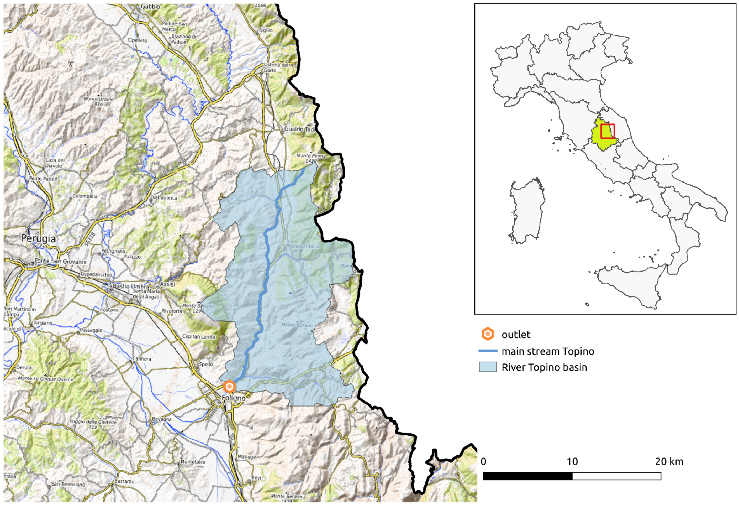
One of the most important rivers in the Umbria region in central Italy is the Topino River, a tributary of the Tiber River. This river belongs to the hydrographic basin of Topino-Marroggia, which incorporates two different basins: the basin of Marroggia-Teverone-Timia and the basin of the Topino River (Figure 2). The Topino River Basin is about 250 km2, with a length of 35 km and an elevation drop of 430 m.
From a geological point of view [15], the River Topino basin is situated almost entirely on the Miocene terrigenous deposits of the “Marnoso-Arenacea” Formation (Umbrian-Marchean Series), which consists of an alternation of marls and sandstones in variable proportions, in the facies of flysch. In its middle valley, the river receives contributions from tributaries that originate from the carbonate reliefs of Mt. Subasio (to the west) and the Foligno Mountains (to the east). The last reach of the Topino forms a wide alluvial fan at its outlet in the Umbrian Valley (Foligno-Spoleto plain) that represents the eastern “branch” of the Ancient Tiberine Lake [16], which was filled during the Pliocene and Pleistocene by clastic sediments in lacustrine and fluvio-lacustrine facies (conglomerates, sands, and clays).
2. Methods
The procedure proposed herein aims to define the value of the TSP at any cross-section of a river using a GIS procedure that is as simple and accurate as possible and based on available data; the particular focus is on the determination of the local slope. Recent available DEMs enable the calculation of the channel gradient and, consequently, the stream power with a finer spatial resolution, and this presents promising and novel opportunities to investigate river geomorphological processes and forms.
Nevertheless, determining the slope remains a difficult task because the evaluation should be as local as possible [17].
The method presented in this section is implemented in a GRASS GIS module called r.stream.power. This code is further described in more detail in Section 2.3.
2.1. Peak Flow Discharge
The estimation of the maximum peak flow at a particular cross-section of a riverbed for a given return period is a problem with a difficult solution because there are many factors involved.
In Italy, the River Tiber Basin Authority proposed a Flood Estimation Handbook, and its purpose was to guide the evaluation of peak flows at any location in the River Tiber Basin [18]. This study used data from 165 gauge stations that are distributed within the basin, and it proposed a methodology that combines the results of analyzing regional precipitation with a duration from 1–24 h with the curve number method [19] to quantify the volume of net rainfall.
The procedure implemented in a GIS environment [14] starts from the calculation of the upslope catchment area by correctly identifying the outlet point for any given point. The calculation code finds the closest point located in the stream network since the point provided by the user cannot be correctly positioned. This point is identified by the r.distance module in GRASS GIS. The extracted stream network is then ordered by Strahler’s stream hierarchy method [20]. A typical operation performed in the reconstruction of the main channel is the application of the vector network analysis tools, in which the outlet point is the starting point of the path. In this approach, the hydrographic network is considered as a road network. In iterating network analysis, when a new main channel needs to be determined, the computational time is substantially increased. The code implemented in this study identifies the main channel by matrix segmentation on the basis of the same algorithms as those used in network analysis. Then, a grid approach is applied by combining the raster of the drainage directions and the raster of the ordered hydrographic network according to Strahler. The procedure is also able to derive other information required for the slope determination, as further explained in the subsection below.
Another expedient that was used to speed up the calculation operations was the calculation of the raster of the hydrographic network (the input required by r.distance) and the flow direction map (necessary for the next step) for the entire Tiber River Basin by means of a digital elevation model. This avoids the need to reprocess these maps at the request of any user.
Starting from the ordered hydrographic network, the code selects the maximum order of the stream network; then, it executes a map algebra operation to extract the main stream, as explained above. This operation enables the calculation of the run-off time using the Kirpich (Equation (2)) or Giandotti method (Equation (3)), depending on the basin area: when the basin area is less than 10 km2, the Kirpich equation is used; otherwise, the Giandotti equation is used.
- Kirpich equation for basins smaller then 10 km2:withTc = run-off time (hours);L = main channel length (km);DH = drop in elevation of the main channel (m).
- Giandotti equation for basins larger than 10 km2:withTc = run-off time (hours);S = basin area (km2);L = main channel length (m);H = mean basin elevation (m a.s.l.).
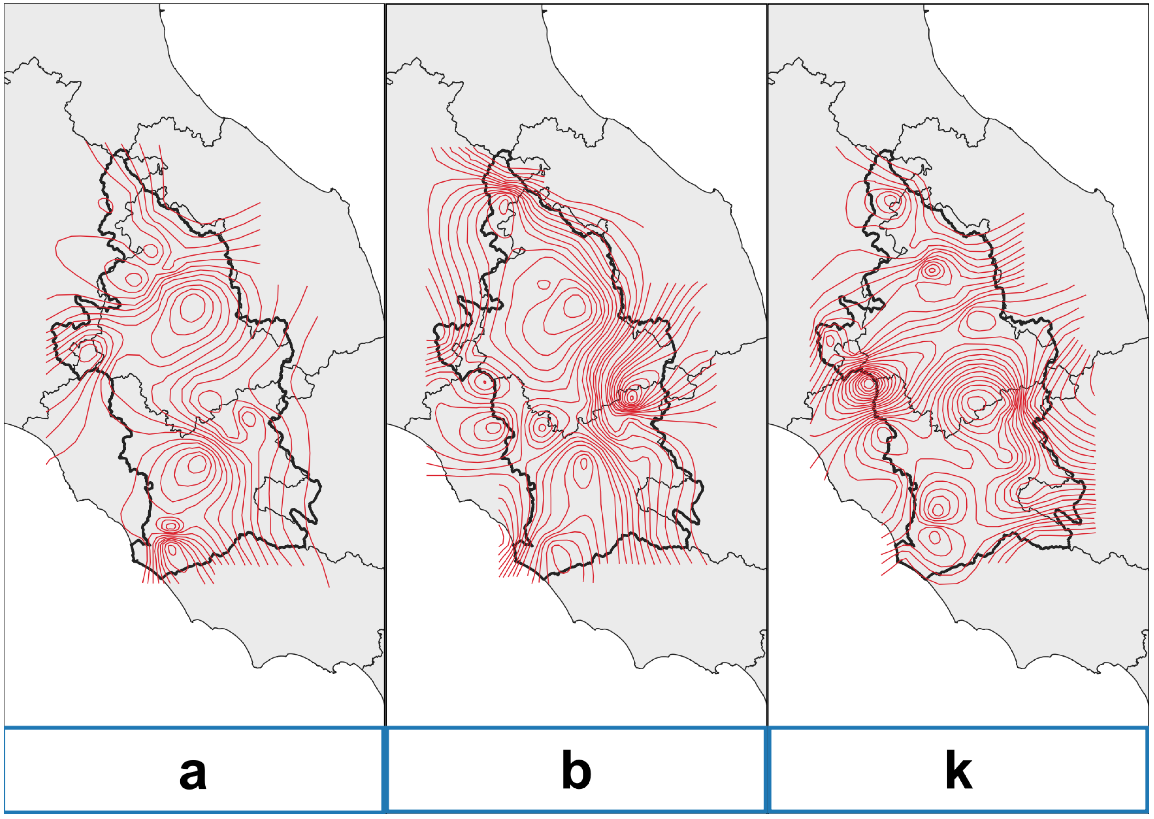
Subsequently, the Intensity-Duration-Frequency (IDF) parameters (a, b, and K) corresponding to the analyzed river basin are calculated. The Flood Estimation Handbook provides several maps to evaluate the IDF parameters (see Figure 3). The GIS procedure derives the values for a, b, and K automatically. This provides a better determination of the aforementioned parameters relative to the standard procedure proposed by the Flood Estimation Handbook. The Handbook proposes the evaluation of IDF parameters using isoline maps at the centroid of the basin; in the GIS procedure, these factors are instead determined as weighted means of the basin.
The maps of IDF parameters (a, b, and K) are used as raster input data of r.stream.power. These raster maps were obtained through a TIN interpolation procedure; the pixel resolution is 25 m, which is the same as the DEM’s resolution. The DEM utilized in this work is the European Digital Elevation Model (EU-DEM), Version 1.1, provided by the European Commission in the Copernicus Project.
Similarly, the Curve Number (CN) is calculated from the raster map previously obtained as the weighted mean value of the basin.
This procedure is implemented in a GIS system, and the GRASS GIS scripts created [21] determine the peak flow rate for each point of the hydrographic network and for the requested return period.
2.2. Slope Determination
Slope determination is a crucial aspect in the evaluation of SP along a reach. A Digital Elevation Model (DEM) represents the starting point to derive the slope map. In GIS, the slope maps are normally obtained using a moving window (3 × 3 in many cases) following the main method available in GIS software, as was carried out by Evans [22] or Zevenbergen and Thorne [23].
Equation (1) requires the determination of the local energy slope S, which can be approximated by the bed slope. The DEM can provide an approximation of the local bed slope.
EU-DEM v1.1 has a planar resolution of 25 m with a vertical accuracy of 2.9 m, as assessed in https://land.copernicus.eu/pan-european/satellite-derived-products/eu-dem. Especially, when it is necessary to calculate the slope for fluvial reaches, the normal proposed approaches are no longer valid [24]. In fact, for the given EU-DEM, it appears that the minimum valuable slope is on the order of:
where is the vertical accuracy.
Therefore, the minimum valuable slope is several orders of magnitude bigger than the floodplain’s river slope, which is around 0.001. For this reason, in this paper, the local slope is not calculated by means of the moving window using the classical GIS approach, but rather by calculating the channel gradient as the ratio between the elevation difference and the real length of the reach.
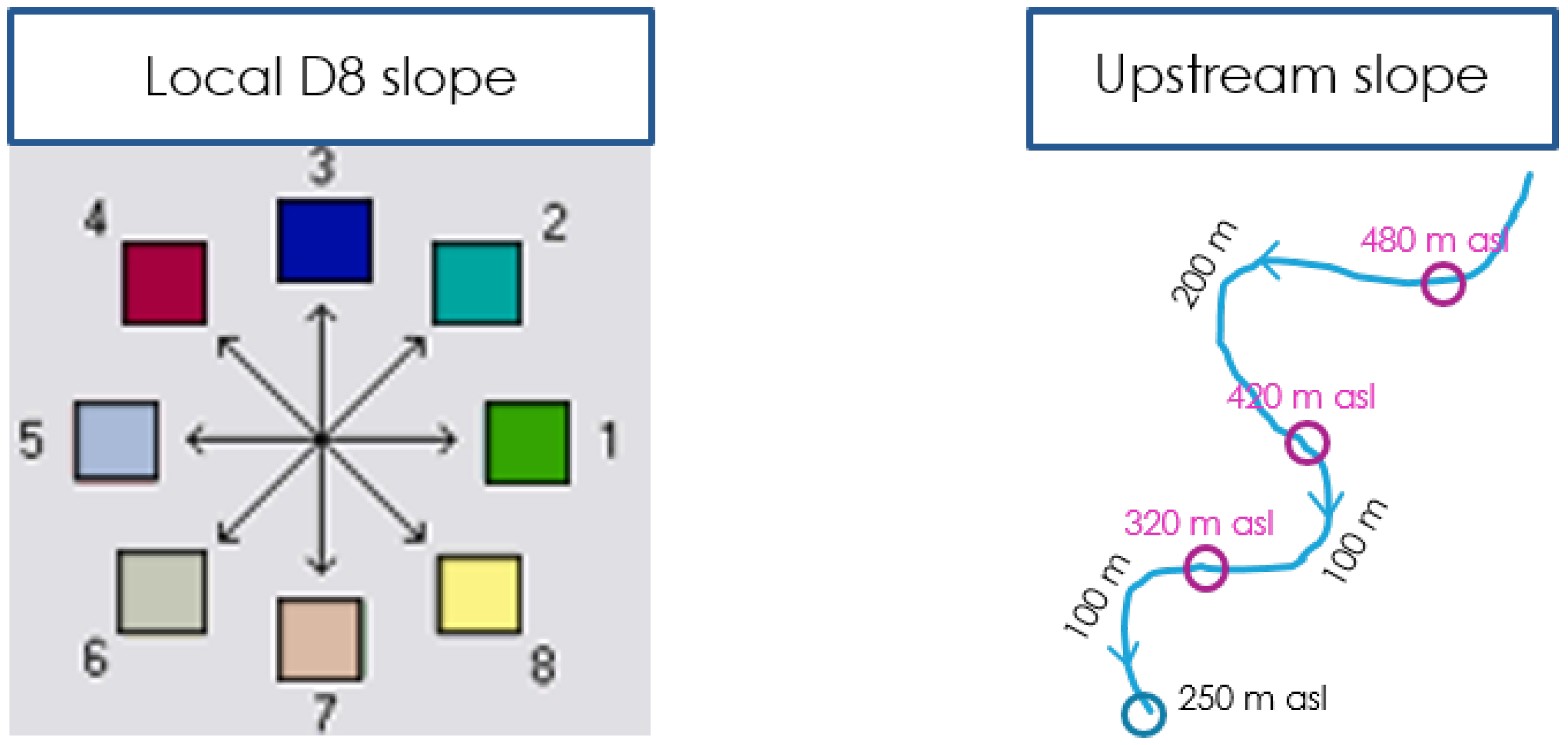
The procedure starts tracking the path of the main channel from the outlet point going upstream following the D8 drainage raster map (Figure 4). Afterward, the cell corresponding to the end of a reach with a certain upstream distance is identified, as shown in Figure 4. In this way, different slopes are obtained according to the upstream reach lengths considered (100, 200, and 400 m). The approach for evaluating the gradient is not present in any of the most common GIS open-source or commercial software packages (GRASS GIS, ARCGIS, SAGA, QGIS, GvSig). Therefore, the implementation of this code represents a novelty of the module that is sure to be of interest for hydrological-hydraulic applications.
The reach length is normally considered to be 20 times the mean width of the riverbed.
2.3. The Module r.stream.power
R.stream.power is a module in GRASS GIS; it is written in Python and able to calculate the stream power quickly at a cross-section of a river network. The code was released under the GNU GPL license, and it is accessible at https://github.com/pierluigiderosa/r.stream.power/releases/tag/1.0. The repository contains the source code of r.stream.powerand a GRASS GIS database with all necessary input data (CN raster map, IDF raster parameters); therefore, the intent here is to provide a fully-reproducible example.
Figure 5 shows the r.stream.power module’s graphical user interface, which clearly shows the required input data: vector points representing the locations of cross-sections at which to calculate the stream power and DEM. No other input is required by the code for determining the flow rate and slope because the additional information (CN and IDF parameters) is automatically determined. In particular, the determination of the CN and IDF parameters is carried out using the weighted average of the CN and IDF rasters (a, b, k), given the contributing upstream area related to the specific cross-section.
The r.stream.power output is a point vector layer that uses an attribute table to store all code-calculated parameters, such as discharge, downstream channel length from the source point, local elevation, elevation drops, upslope for several distances, and the TSP for upslope distances of 100, 200, 400 m.
The module introduces two novel elements to the stream power calculation: (1) a hydro-morphological rigorous approach for the evaluation of the local slope upstream at a given cross-section (see Section 2.2); (2) here, the flow rate, which is normally calculated with a discharge-area equation [2,25,26], is determined with more detail, i.e., spatial rainfall distribution and infiltration (using the Curve Number method) are also incorporated.
3. Results
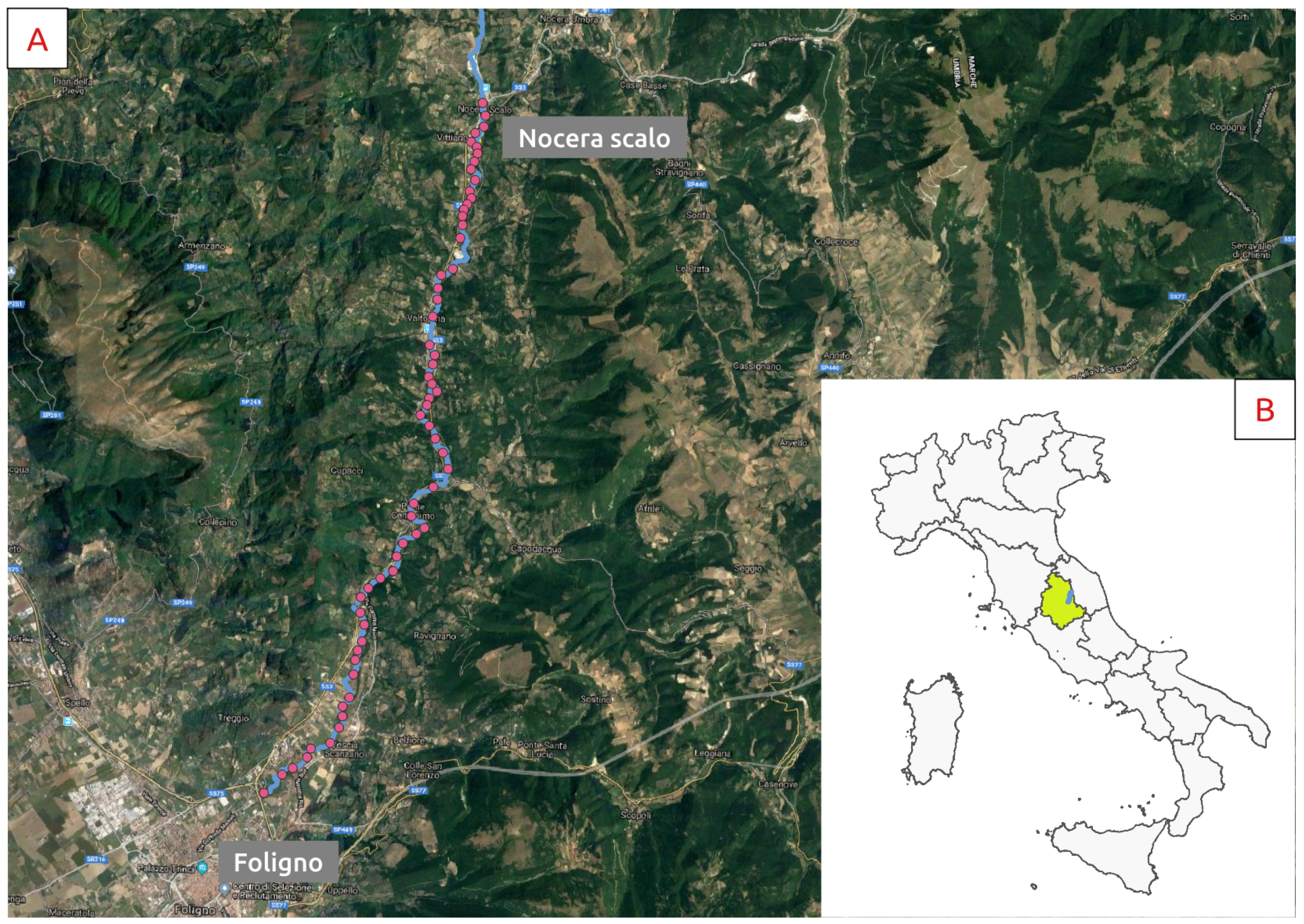
First, this work used GRASS GIS for the calculation of the precise flow values related to 62 points identified along the Topino River from the confluence of Caldognola Creek, which is close to the town of Nocera Umbra (Nocera Scalo), up to the entrance of the river near Foligno, as shown in Figure 6. These points are located along the hydrographic network of the river under study and are approximately spaced by a distance that is about 20-times the mean width of the riverbed. Subsequently, the slope values (S) of the channel were determined following the method described in the section above.
Therefore, the river was split into 61 sections of the reach; any reach has a length of about 20-times the mean-width channel. At the end of each reach, once the necessary data (mean flow and relative slope of each section) were evaluated, Equation (1) proposed by Bagnold [1] was applied.
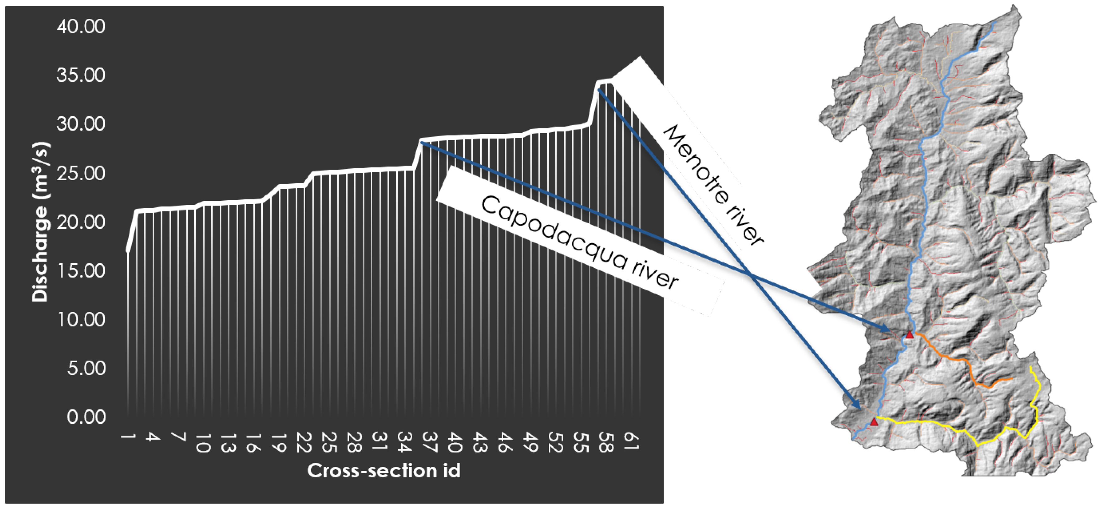
The discharge values corresponding to 62 cross-sections are shown in Table 1, and they ranged between a minimum value of 17.1 m3/s and a maximum value of 35.2 m3/s.
The discharges listed in Table 1 are plotted in Figure 7. The discharge presents two big increments: the major one, which corresponds to the confluence of an important tributary (Menotre River); the second one, which corresponds to the confluence of a small river coming from the left, close to the outlet of the Topino Basin.
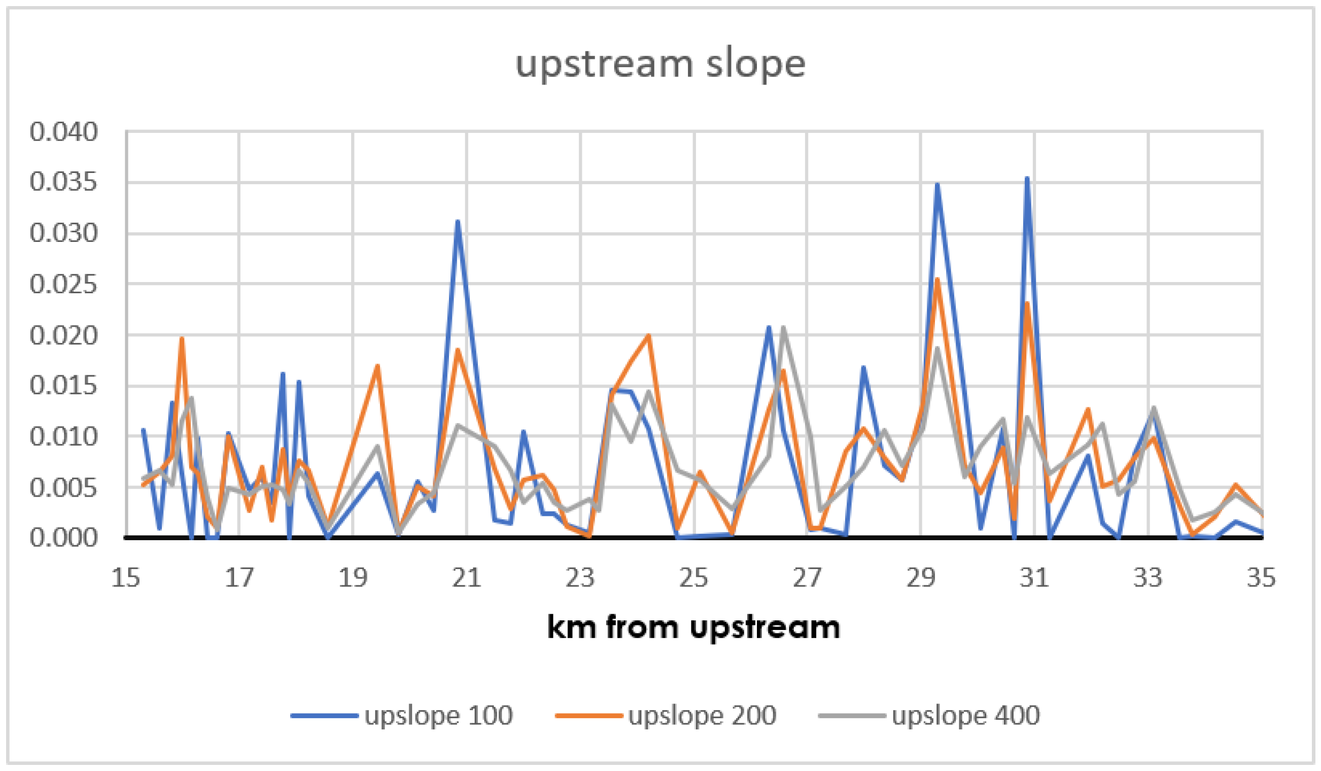
As explained in the section above, for each cross-section, the slope was calculated as the ratio of the drop for a certain distance upstream of the cross-section to the distance itself. Figure 8 shows the variation in the upstream slope along the reach of the Topino River. Figure 8 suggests that carrying out the calculations by increasing the upstream distances from the cross-section from 100–400 m leads to lower slope values. The slope calculated at greater distances was smoother than the one calculated at 100 m. However, the changes in the slope responsible for the variations (increases or decreases) in the stream power were present in all the drops.
Table 2 reports the Total Stream Power (TSP) values calculated for all cross-sections, expressed in W/m; the values in bold correspond to the highest values, which are further described below.
In Table 2, the zero values of the TSP at an upslope distance of 100 m were a result of the low accuracy of the DEM. Moving only 100 m upslope from the current outlet did not change the elevation value, so the drop was equal to zero.
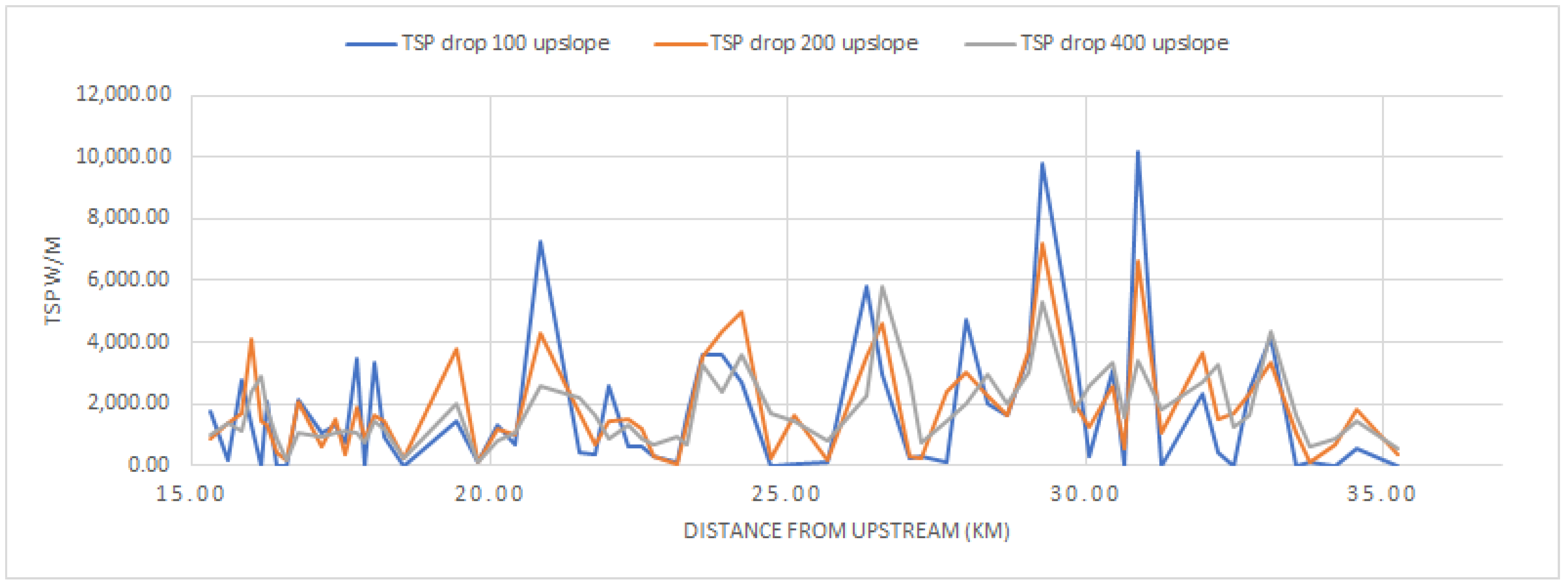
Figure 9 shows the variation in the TSP in the studied reach of the Topino River. The figure plots the TSP values calculated using the slopes determined at upstream distances of 100 m, 200 m, and 400 m. The gray line represents the TSP obtained from the elevation drop at 400 m upstream and is smoother compared with the TSP obtained at 100 m upstream.
4. Discussion
Starting from the TSP definition in Equation (1), a high TSP value could be related to a high value of the local slope, a high value of discharge, or both. In these cases, at the points where the TSP increases, a higher value of potential stream energy is available that the river uses for sediment transport and erosion processes. Local peaks in TSP are thus related to local river morphological features.
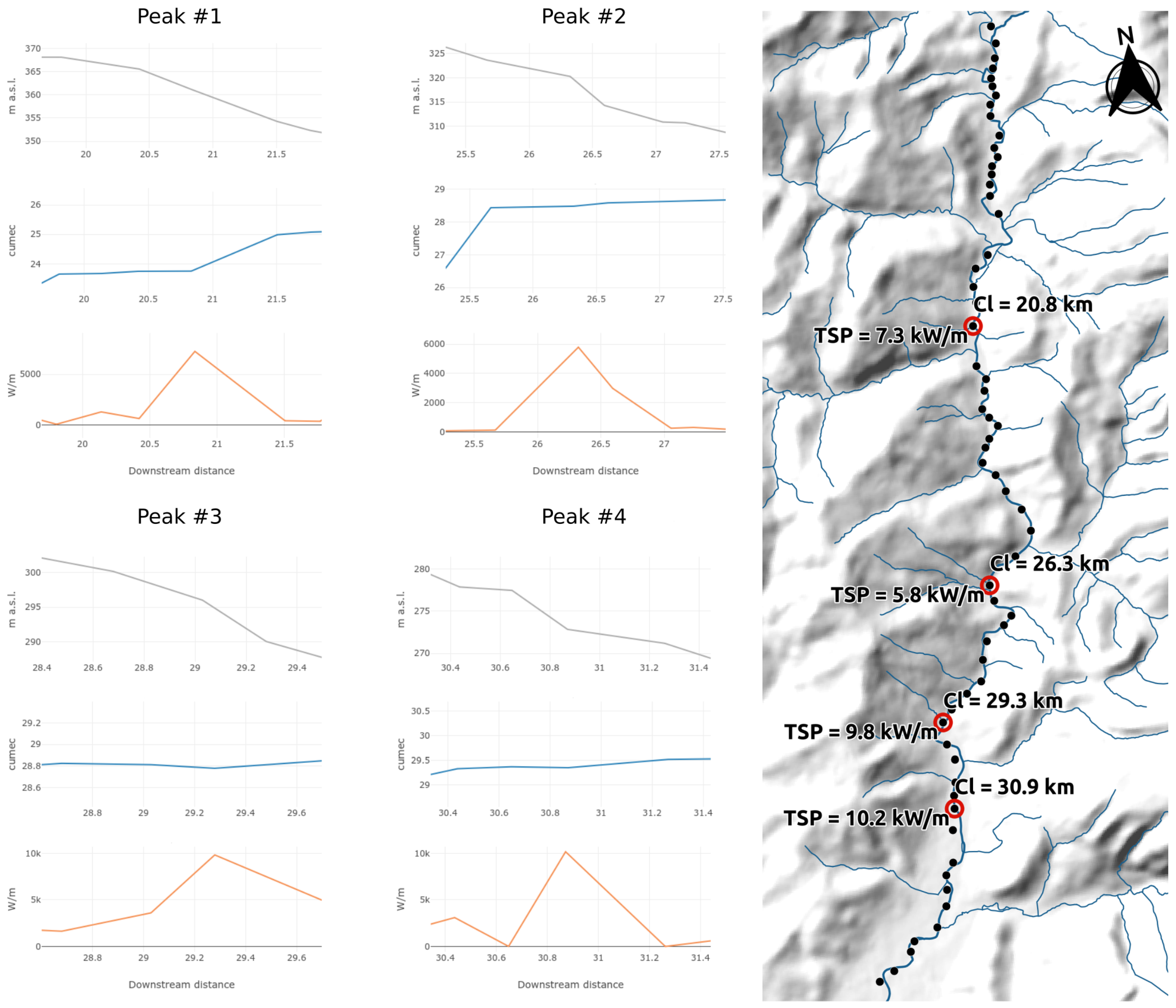
The trend of the TSP shown in Table 2 and in Figure 9 reveals that there were some clear peaks along the studied river. Some other high values of TSP were present, although they were not as prominent.
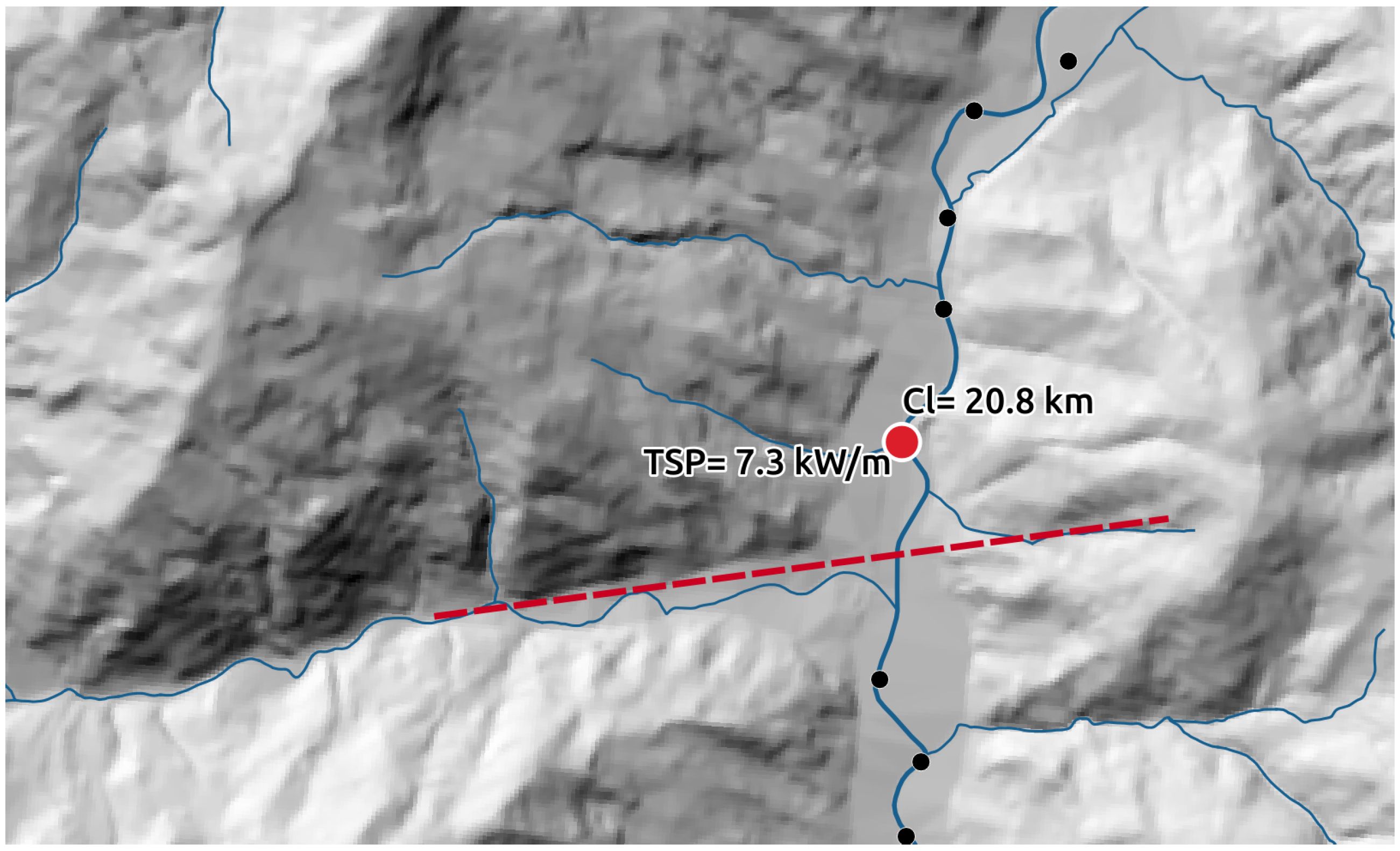
- Peak #1 is located 20.8 km downstream with a TSP value of 7250 W/m for an upslope distance of 100 m, 4295 W/m for an upslope distance of 200 m, and 2584 W/m for an upslope distance of 400 m. In this cross-section, the high value of the TSP was due to the local slope (about 1.8%) and discharge.
- Peak #2 is located 26.3 km downstream; the TSP ranged from 2270 W/m (for an upslope distance of 400 m) to 5796 W/m (for an upslope distance of 100 m). Even in this case, the increase in TSP was caused by high values of the discharge (the discharge increased from 25.5 m3/s–28.4 m3/s) and local slope (about 1–2%). In this section, in fact, the Rio Capodacqua, with its 35-km2 watershed, flows into the Topino River.
- Peak #3 is located 28.7 km downstream, with a TSP that ranged from 5286 W/m–9821 W/m. In this cross-section, the increase in the TSP was related to high values of the local slopes (about 3.5%).
- Peak #4 is located 29.3 km downstream with a TSP that ranged from 3429 W/m–10,164 W/m. Even here, the TSP increase was related to high values of the local slopes (about 3.5%).It is interesting to analyze the causes of a local gradient increase highlighted in Figure 10. Generally, high slope values are due to geological structural elements. For Peak # 1, the high value of SP was partially due to an increase in the flow discharge. Nevertheless, geological surveying demonstrated that this value of SP was due to the overall presence of a fault, which was evident by the alignment of the tributaries (on the right and on the left) of the Topino River (see Figure 11). The fault produced a clear increase in the Topino River slope as a consequence of the regressive erosion of the main channel that tried to re-establish its equilibrium profile. Furthermore, Peak # 2 is interesting because it showed the same situation: the increase in the slope was produced by a normal fault that caused a nick-point in the river longitudinal profile. It is likely that the fault activity was fairly recent because the river had not yet regulated the longitudinal profile to an equilibrium condition, resulting in a nick-point that was more evident than that in the previous case. Figure 12b shows the DEM, in which the fault appears clearly and produces an escarpment; this is also confirmed by the Geological Map of Italy (a), which displays a system of three faults in the same area. In order to determine the riverbed conditions in the locations of Peaks #3 and #4, a field survey was carried out. The survey revealed that the riverbed located upstream of these points is characterized by a step-pool morphology [27] that is related to the bedrock outcropping. Furthermore, in this reach, which is located at the entrance of a wide alluvial plain, the slope of the riverbed is controlled by the bedrock setting.
The code implemented used several optimizations in order to reduce the computational time as much as possible. r.stream.power was already working in a reasonable CPU time before the code optimization; analyzing 62 points with a mean of 30 km2 of the upstream contributing basin took about 25 min. For each cross-section, the initial code version calculated the hydrographic network, which was then ordered by Strahler’s method [20], and extracted the main channel and the upstream contributing basin. Subsequently, it determined the average value of CN and the IDF parameters necessary to evaluate the discharge. Nevertheless, an analysis of the computational times of various parts of code was performed; the results indicated that the operations that required more CPU time were the determination of the hydrographic network and the analysis of the networks used to derive the main channel. The current optimized code calculated the hydrographic network and the map of the drainage directions only once for the entire area analyzed by the DEM; later, for each cross-section, the whole network was cut out on a smaller region and ordered by the Strahler method [20]. The main channel was therefore identified by matrix segmentation on the basis of the network analysis algorithm, but using the grid approach, combining the raster of the drainage directions and the raster of the Strahler-ordered hydrographic network. This grid network analysis approach reduced the calculation time. The optimized code, with the same hardware, took about 10 min to analyze the same 62 points.
Of course, the best way to reduce the computational time considerably was to run these operations in parallel with the calculation process. Such a feature could be easily developed as, for a specific cross-section, the total stream power calculation is independent of any other cross-sections.
5. Conclusions
In this study, the equation proposed by Bagnold [1] related to stream power was used to analyze the variation in its values along a river and its relation with fluvial dynamics. The Stream Power (SP) represents the dissipation of the potential energy per unit of channel length, and it is obtained by the product of the flow rate (m3/s), the slope of the channel (m/m), the density (kg/m3), and the gravitational acceleration (m/s2). It is therefore expressed in W/m and can be considered as a measure of the main driving forces acting within a channel, thus influencing the capability of a stream to transport sediments.
This work shows how the determination of SP values can provide useful indications of the dynamics of river processes. It is clear that a large-scale analysis within a river basin could indicate, in a preventive and forecasting way, the areas most “sensitive” to changes, as they are potentially subject to instability phenomena caused by the fluvial dynamics.
This study proposed a GRASS GIS code for the fast and local estimation of the Total Stream Power (TSP). The flow discharge estimation is one of the main challenges in TSP determination; deriving the flow discharge directly using only cross-section location as input is a hard task. In this work, the approach proposed by the Flood Estimation Handbook published by the River Tiber Basin Authority was implemented [14]. Subsequently, the channel gradient was obtained from a DEM using the elevation drop between a cell and the cell upstream at distances of 100 m, 200 m, and 400 m, as proposed by Bizzi and Lerner [12].
The module called r.stream.power is freely available ((https://github.com/pierluigiderosa/r.stream.power/releases/tag/1.0). The repository also contains all necessary input data (CN raster map of Umbria and IDF raster parameters for the Tiber River Basin). r.stream.power presents two novel elements in the stream power calculation: (1) a hydro-morphological rigorous approach for the evaluation of the local slope upstream in a given cross-section; (2) the flow rate, frequently calculated with a discharge-area equation, is determined considering spatial rainfall distribution and infiltration by the mean value of the curve number for the upstream contributing basin.
The method was tested on a case study, the Topino River (Umbria, Central Italy), using the portion starting from the confluence with Caldognola Creek, which is close to the town of Nocera Umbra (Nocera Scalo), until the town of Foligno. The analyzed portion of the Topino River has a narrow and longitudinally-discontinuous alluvial plain (partly confined valley [9]). Furthermore, the riverbed has undergone vertical erosion, and it now flows directly on the bedrock. The SP and discharge variations are influenced by these conditions, mainly by the bedrock setting and tectonic features.
The variations in SP appears to be strongly correlated with the geomorphological and geological structure characteristics, especially for fixed rivers: increases in SP values have been demonstrated as the analysis of the variations in this parameter can be utilized to detect areas influenced by tectonic features (i.e., faults) due to the “accommodation” of the river dynamics to the geological assessment.
Author Contributions
P.D.R. implemented the Python code and tested the application. P.R.D. performed the runs. P.D.R. and A.F. tested the results. C.C. provides the geomorphological interpretations. All authors wrote the paper.
Funding
This research received no external funding.
Conflicts of Interest
The authors declare no conflict of interest.
Abbreviations
The following abbreviations are used in this manuscript:
| DEM | Digital Elevation Model |
| TSP | Total Stream Power |
| SP | Stream Power |
| IDF | Intensity-Duration-Frequency curve |
| TIN | triangulated irregular network |
References
- Bagnold, R.A. An Approach to the Sediment Transport Problem From General Physics; US Government Printing Office: Washington, DC, USA, 1966.
- Jain, V.; Preston, N.; Fryirs, K.; Brierley, G. Comparative assessment of three approaches for deriving stream power plots along long profiles in the upper Hunter River catchment, New South Wales, Australia. Geomorphology 2006, 74, 297–317. [Google Scholar] [CrossRef]
- Barker, D.M.; Lawler, D.M.; Knight, D.W.; Morris, D.G.; Davies, H.N.; Stewart, E.J. Longitudinal distributions of river flood power: the combined automated flood, elevation and stream power (CAFES) methodology. Earth Surf. Process. Landf. 2009, 34, 280–290. [Google Scholar] [CrossRef]
- Bagnold, R. Bed load transport by natural rivers. Water Resour. Res. 1977, 13, 303–312. [Google Scholar] [CrossRef]
- Nanson, G.; Croke, J. A genetic classification of floodplains. Geomorphology 1992, 4, 459–486. [Google Scholar] [CrossRef] [Green Version]
- Ferguson, R. Estimating critical stream power for bedload transport calculations in gravel-bed rivers. Geomorphology 2005, 70, 33–41. [Google Scholar] [CrossRef]
- Comiti, F.; Mao, L. Recent advances in the dynamics of steep channels. Gravel-Bed Rivers: Processes, Tools, Environments; John Wiley & Sons: Hoboken, NJ, USA, 2012; pp. 351–377. [Google Scholar]
- Knighton, A. Downstream variation in stream power. Geomorphology 1999, 29, 293–306. [Google Scholar] [CrossRef]
- Brierley, G.J.; Fryirs, K.A. Geomorphology and River Management: Applications of the River Styles Framework; Blackwell Publishing: Hoboken, NJ, USA, 2005. [Google Scholar]
- Church, M.; Hassan, M.A. Size and distance of travel of unconstrained clasts on a streambed. Water Resour. Res. 1992, 28, 299–303. [Google Scholar] [CrossRef]
- Tsutsumi, D.; Laronne, J.B. Gravel-Bed Rivers: Process and Disasters; John Wiley & Sons: Hoboken, NJ, USA, 2017. [Google Scholar]
- Bizzi, S.; Lerner, D. The use of stream power as an indicator of channel sensitivity to erosion and deposition processes. River Res. Appl. 2015, 31, 16–27. [Google Scholar] [CrossRef]
- Vocal Ferencevic, M.; Ashmore, P. Creating and evaluating digital elevation model-based stream-power map as a stream assessment tool. River Res. Appl. 2012, 28, 1394–1416. [Google Scholar] [CrossRef]
- De Rosa, P.; Fredduzzi, A.; Minelli, A.; Cencetti, C. Automatic Web Procedure for Calculating Flood Flow Frequency. Water 2019, 11, 14. [Google Scholar] [CrossRef]
- Cencetti, C. Morfotettonica ed evoluzione plio/pleistocenica del paesaggio nell’area appenninica compresa tra i monti di Foligno e la Val Nerina (Umbria centro-orientale). Boll. Soc. Geol. Ital. 1993, 112, 235–250. [Google Scholar]
- Albani, A. L’antico lago tiberino. L’Universo 1962, 52, 731–750. [Google Scholar]
- Robert, A. River Processes: An Introduction to Fluvial Dynamics; Routledge: Abingdon, UK, 2014. [Google Scholar]
- Autorita di Bacino del Fiume Tevere. Quaderno Idrologico del Fiume Tevere. Tevere 1996, 1, 64. [Google Scholar]
- Cronshey, R. Urban Hydrology for Small Watersheds, 2nd ed.; Technical Report; U.S. Dept. of Agriculture, Soil Conservation Service, Engineering Division: Washington, DC, USA, 1986.
- Strahler, A.N. Quantitative analysis of watershed geomorphology. Eos Trans. Am. Geophys. Union 1957, 38, 913–920. [Google Scholar] [CrossRef]
- De Rosa, P. r.stream.power: v1.0, Zenodo April 2019. Available online: https://zenodo.org/record/1463784#.XPCfZYh5tPY (accessed on 31 May 2019).
- Evans, I.S. General Geomorphometry, Derivatives of Altitude, and Descriptive Statistics; Chorley, R.J., Ed.; Spatial Analysis in Geomorphology: Methuen, MA, USA, 1972; pp. 17–90. [Google Scholar]
- Zevenbergen, L.W.; Thorne, C.R. Quantitative analysis of land surface topography. Earth Surf. Process. Landf. 1987, 12, 47–56. [Google Scholar] [CrossRef]
- Hengl, T.; Reuter, H. (Eds.) Geomorphometry: Concepts, Software, Applications; Elsevier: Amsterdam, The Netherlands, 2008; Volume 33, p. 772. [Google Scholar]
- Pérez-Peña, J.V.; Azañón, J.M.; Azor, A.; Delgado, J.; González-Lodeiro, F. Spatial analysis of stream power using GIS: SLk anomaly maps. Earth Surf. Process. Landf. 2009, 34, 16–25. [Google Scholar] [CrossRef]
- Finlayson, D.P.; Montgomery, D.R. Modeling large-scale fluvial erosion in geographic information systems. Geomorphology 2003, 53, 147–164. [Google Scholar] [CrossRef]
- Montgomery, D.R.; Buffington, J.M. Channel-reach morphology in mountain drainage basins. Geol. Soc. Am. Bull. 1997, 109, 596–611. [Google Scholar] [CrossRef]
Figure 1.
Schematic representation of the relationship between downstream changes along a river and associated transitions in sediment process. Source: https://extension.umass.edu/riversmart/sites/extension.umass.edu.riversmart/files/fact-sheets/pdf/Task_Force_StreamPower.pdf.
Figure 1.
Schematic representation of the relationship between downstream changes along a river and associated transitions in sediment process. Source: https://extension.umass.edu/riversmart/sites/extension.umass.edu.riversmart/files/fact-sheets/pdf/Task_Force_StreamPower.pdf.

Figure 2.
Hydrographic basin of Topino. The blue line represents the Topino River. The red rectangle on the right represents the coverage area.
Figure 2.
Hydrographic basin of Topino. The blue line represents the Topino River. The red rectangle on the right represents the coverage area.

Figure 3.
Values of Intensity-Duration-Frequency parameters a, b, and K expressed as isolines, provided by the Flood Estimation Handbook for the whole Tiber River Basin.
Figure 3.
Values of Intensity-Duration-Frequency parameters a, b, and K expressed as isolines, provided by the Flood Estimation Handbook for the whole Tiber River Basin.

Figure 4.
On the left: D8 drainage map definition. Each cell has a value between one and eight in order to identify the water-contributing cell. On the right: reach identification for several stream distances from the outlet point. The algorithm identifies three points (purple circles) along the stream channel: 100, 200, and 400 m upstream from the outlet (blue circle). For each point, the elevation is determined, and then, the elevation drop relative to the outlet point is calculated.

Figure 5.
(A) The user interface of the r.stream.power, the module of GRASS GIS. Required inputs are vector points that represent the locations of cross-sections at which the stream power and DEM should be calculated. (B) The model output represented by a vector points layer; the attribute table contains, in detail, all of the code-calculated parameters, such as discharge, downstream channel length from the source point, local elevation, elevation drops, upslope for several distances, and the TSP for upslope distances of 100, 200, and 400 m. (C) Output points generated by the code plotted over the DEM used as input.

Figure 6.
(A) Identification of points along the studied reach of Topino River (from Google Hybrid). (B) Visualization of the Umbrian region overlapped by the Topino River main channel.
Figure 6.
(A) Identification of points along the studied reach of Topino River (from Google Hybrid). (B) Visualization of the Umbrian region overlapped by the Topino River main channel.

Figure 7.
The line plot’s vertical axis is the discharge, and its horizontal axis is the upstream distance. The steps represent increases in discharge due to confluences. The arrows highlight the correspondence between the steps and the location in the map.
Figure 7.
The line plot’s vertical axis is the discharge, and its horizontal axis is the upstream distance. The steps represent increases in discharge due to confluences. The arrows highlight the correspondence between the steps and the location in the map.

Figure 8.
Plot of the upstream slope calculated using the three distances from the upstream.

Figure 9.
Linear representation for the stream power values along the reach of the Topino River.

Figure 10.
The left part of the figure shows the line plots for the elevation profile (in gray), discharge (in blue), and TSP 100 m upstream (in orange) for Peaks #1–4. On the right, the map shows the location for the four peaks; the label reports the downstream Channel length (Cl) and the TSP expressed in KW/m.

Figure 11.
Peak #1 location. The presence of a fault (red dashed line) is highlighted by the alignment of the two tributaries on the right and left bank.
Figure 11.
Peak #1 location. The presence of a fault (red dashed line) is highlighted by the alignment of the two tributaries on the right and left bank.

Figure 12.
Peak #2 location. (a) shows an extract of the Geological Map of Italy at a scale of 1:100,000 (link: http://www.isprambiente.gov.it/en/cartography/geological-and-geothematic-maps/geological-map-at-a-scale-1-to-100000, last access 04 April 2019) that displays a system of three faults; in (b), details of the DEM where the fault appears are clearly shown.


Table 1.
Values for the peak flow discharge corresponding to the 62 cross-sections along the Topino River.
Table 1.
Values for the peak flow discharge corresponding to the 62 cross-sections along the Topino River.
| No Point | Q (m3/s) | No Point | Q (m3/s) | No Point | Q (m3/s) |
|---|---|---|---|---|---|
| 1 | 17.09 | 22 | 25.08 | 43 | 28.78 |
| 2 | 21.16 | 23 | 25.1 | 44 | 28.87 |
| 3 | 21.19 | 24 | 25.15 | 45 | 29.37 |
| 4 | 21.35 | 25 | 25.22 | 46 | 29.35 |
| 5 | 21.49 | 26 | 25.25 | 47 | 29.73 |
| 6 | 21.35 | 27 | 25.32 | 48 | 30.14 |
| 7 | 21.49 | 28 | 25.35 | 49 | 34.25 |
| 8 | 21.52 | 29 | 25.37 | 50 | 23.75 |
| 9 | 21.55 | 30 | 25.49 | 51 | 24.99 |
| 10 | 21.9 | 31 | 25.47 | 52 | 28.81 |
| 11 | 21.94 | 32 | 25.5 | 53 | 29.33 |
| 12 | 21.98 | 33 | 25.52 | 54 | 28.91 |
| 13 | 22.01 | 34 | 28.44 | 55 | 29.52 |
| 14 | 22.05 | 35 | 28.48 | 56 | 29.56 |
| 15 | 22.07 | 36 | 28.58 | 57 | 29.78 |
| 16 | 22.12 | 37 | 28.64 | 58 | 34.42 |
| 17 | 22.19 | 38 | 28.67 | 59 | 34.5 |
| 18 | 22.81 | 39 | 28.71 | 60 | 34.81 |
| 19 | 23.66 | 40 | 28.74 | 61 | 34.78 |
| 20 | 23.68 | 41 | 28.78 | 62 | 35.2 |
| 21 | 23.76 | 42 | 28.83 |
Table 2.
Values for the total stream power corresponding to the 62 cross-sections along the Topino River, expressed in W/m. Values in bold correspond to the highest values of TSP
Table 2.
Values for the total stream power corresponding to the 62 cross-sections along the Topino River, expressed in W/m. Values in bold correspond to the highest values of TSP
| ID | TSP Upslope Dist. 100 | TSP Upslope Dist. 200 | TSP Upslope Dist. 400 | ID | TSP Upslope Dist. 100 | TSP Upslope Dist. 200 | TSP Upslope Dist. 400 |
|---|---|---|---|---|---|---|---|
| 1 | 1775.82 | 887.91 | 995.82 | 32 | 3608.26 | 4333.66 | 2399.58 |
| 2 | 205.99 | 1369.75 | 1384.04 | 33 | 2693.06 | 4964.72 | 3617.26 |
| 3 | 2769.71 | 1689.04 | 1100.74 | 34 | 0 | 250.13 | 1671.12 |
| 4 | 1326.44 | 4088.01 | 2411.14 | 35 | 42.63 | 1630.99 | 1451.47 |
| 5 | 0 | 1471.07 | 2867.31 | 36 | 119.69 | 162.86 | 807.56 |
| 6 | 2067.75 | 1346.1 | 1824.74 | 37 | 5796.88 | 3530.41 | 2270.71 |
| 7 | 0 | 448.75 | 861.29 | 38 | 2983.37 | 4600.51 | 5792.17 |
| 8 | 0 | 211.09 | 175.19 | 39 | 246.54 | 304.04 | 2829.07 |
| 9 | 2169.69 | 2102.67 | 1051.34 | 40 | 304.25 | 273.83 | 772.59 |
| 10 | 1047.39 | 591.07 | 939.22 | 41 | 92.13 | 2409.56 | 1426.75 |
| 11 | 1307.58 | 1508.62 | 1095.74 | 42 | 4715.52 | 3019.24 | 1995.68 |
| 12 | 759.92 | 379.96 | 1124.67 | 43 | 2041.43 | 2245.54 | 2992.93 |
| 13 | 3487.96 | 1899.82 | 1050.22 | 44 | 1635.87 | 1635.79 | 2044.76 |
| 14 | 0 | 873.71 | 746.66 | 45 | 3603.57 | 3704.33 | 3031.84 |
| 15 | 3310.11 | 1655.06 | 1453.99 | 46 | 9821.8 | 7197.84 | 5286.04 |
| 16 | 914.71 | 1443.87 | 1189.17 | 47 | 4047.69 | 2050.47 | 1733.87 |
| 17 | 0 | 247.75 | 222.36 | 48 | 282.32 | 1285.76 | 2584.99 |
| 18 | 1429.41 | 3776.96 | 2036.58 | 49 | 3098.73 | 2560.6 | 3354.75 |
| 19 | 94.62 | 122.98 | 108.78 | 50 | 9.58 | 585.33 | 1574.71 |
| 20 | 1306.47 | 1197.6 | 795.25 | 51 | 10,164.98 | 6626.91 | 3429.73 |
| 21 | 655.28 | 982.88 | 1037.49 | 52 | 0 | 1086.14 | 1852.62 |
| 22 | 7250.18 | 4295.24 | 2584.58 | 53 | 2347.07 | 3659.51 | 2685.01 |
| 23 | 439.89 | 1691.53 | 2212.57 | 54 | 453.54 | 1496.99 | 3277.99 |
| 24 | 383.8 | 698.94 | 1648.99 | 55 | 0 | 1696.03 | 1249.72 |
| 25 | 2587.56 | 1424.29 | 888.19 | 56 | 2438.49 | 2342.2 | 1659.04 |
| 26 | 599.21 | 1527.07 | 1335.6 | 57 | 4187.26 | 3312.15 | 4336.91 |
| 27 | 618.92 | 1187.67 | 894.58 | 58 | 0 | 1092.1 | 1648.86 |
| 28 | 323.93 | 277.71 | 668.05 | 59 | 100.86 | 110.93 | 607.85 |
| 29 | 136.88 | 68.44 | 959.4 | 60 | 0 | 704.58 | 861.7 |
| 30 | 1615.29 | 1383.2 | 691.6 | 61 | 584.78 | 1793.74 | 1474.23 |
| 31 | 3611.47 | 3522.19 | 3252.77 | 62 | 0 | 378.64 | 589.71 |
© 2019 by the authors. Licensee MDPI, Basel, Switzerland. This article is an open access article distributed under the terms and conditions of the Creative Commons Attribution (CC BY) license (http://creativecommons.org/licenses/by/4.0/).
Share and Cite
MDPI and ACS Style
De Rosa, P.; Fredduzzi, A.; Cencetti, C. Stream Power Determination in GIS: An Index to Evaluate the Most ’Sensitive’Points of a River. Water 2019, 11, 1145. https://doi.org/10.3390/w11061145
AMA Style
De Rosa P, Fredduzzi A, Cencetti C. Stream Power Determination in GIS: An Index to Evaluate the Most ’Sensitive’Points of a River. Water. 2019; 11(6):1145. https://doi.org/10.3390/w11061145
Chicago/Turabian StyleDe Rosa, Pierluigi, Andrea Fredduzzi, and Corrado Cencetti. 2019. "Stream Power Determination in GIS: An Index to Evaluate the Most ’Sensitive’Points of a River" Water 11, no. 6: 1145. https://doi.org/10.3390/w11061145
Note that from the first issue of 2016, this journal uses article numbers instead of page numbers. See further details here.