Analysing the Near-Field Effects and the Power Production of Near-Shore WEC Array Using a New Wave-to-Wire Model

 ,
,  , , , and
Abstract
:1. Introduction
- coupling between the BEM solver NEMOH and the mild-slope wave propagation model MILDwave,
- development of an iterative technique to model WEC Farms composed of clustered WEC arrays,
- development of a realistic time-domain Power Take-off (PTO) module.
- a wave climate representative of that observed at the installation site,
- a realistic sloping bathymetry,
- a WEC with approximate dimensions to the WEC technology that is to be deployed,
- a hydraulic PTO system simulating that of the proposed WEC,
- a WEC farm layout that seeks to maximize power absorption over a limited coastal length.
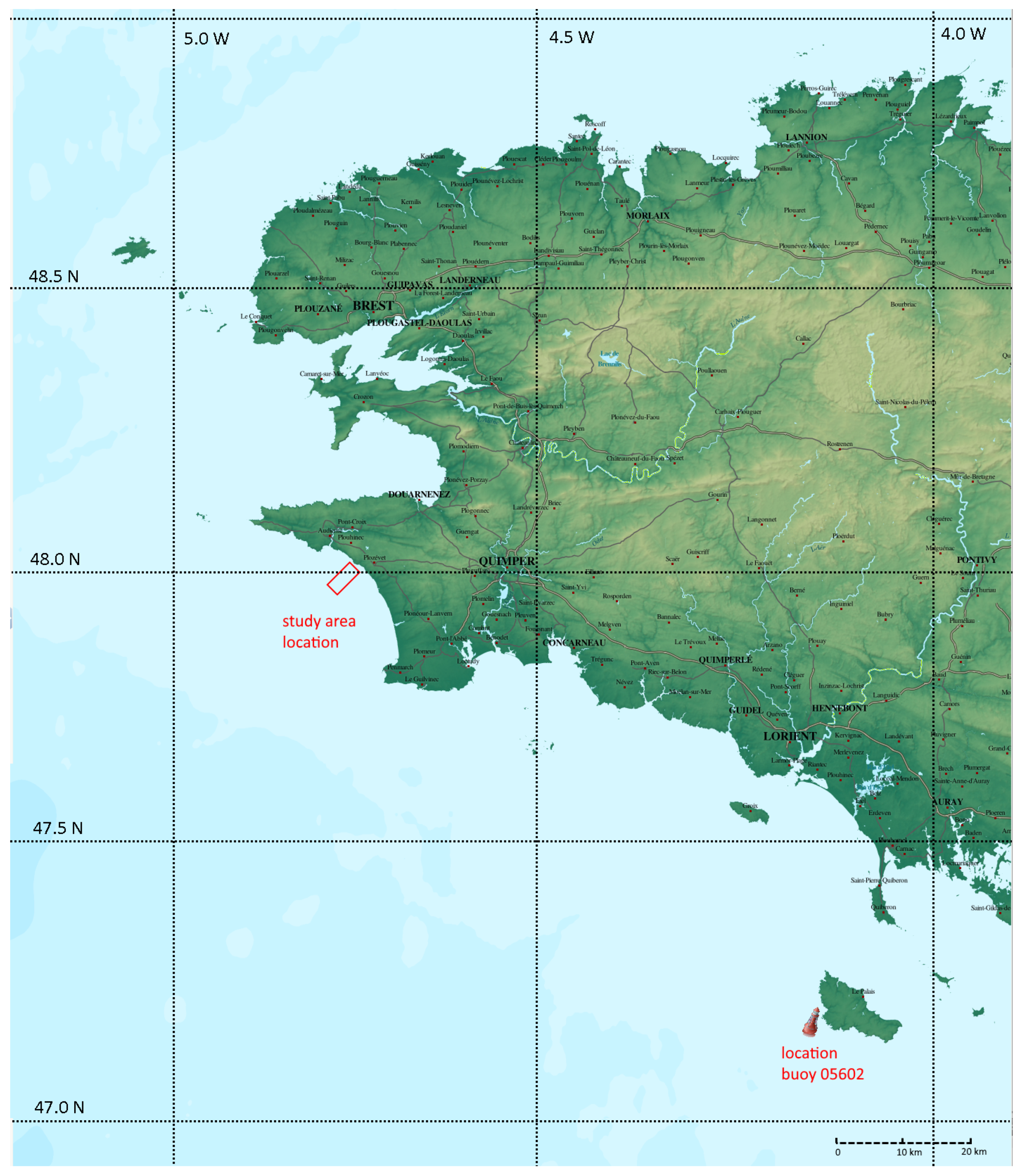
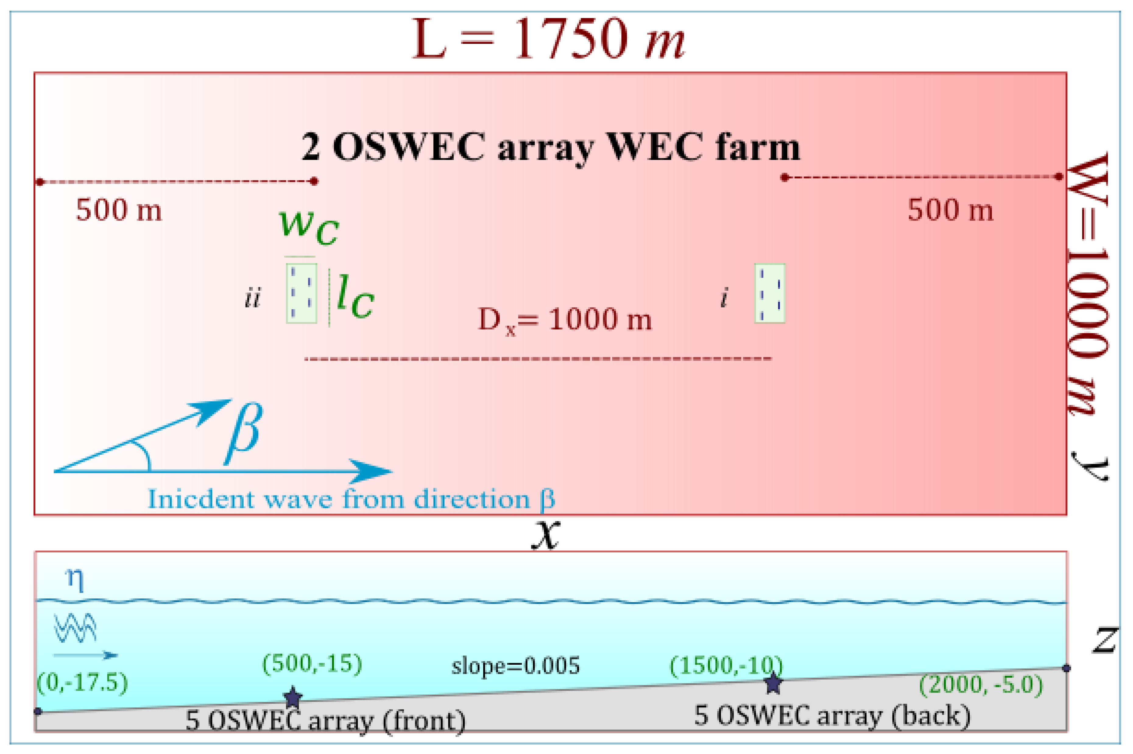
1.1. Study Location and Geographical Context
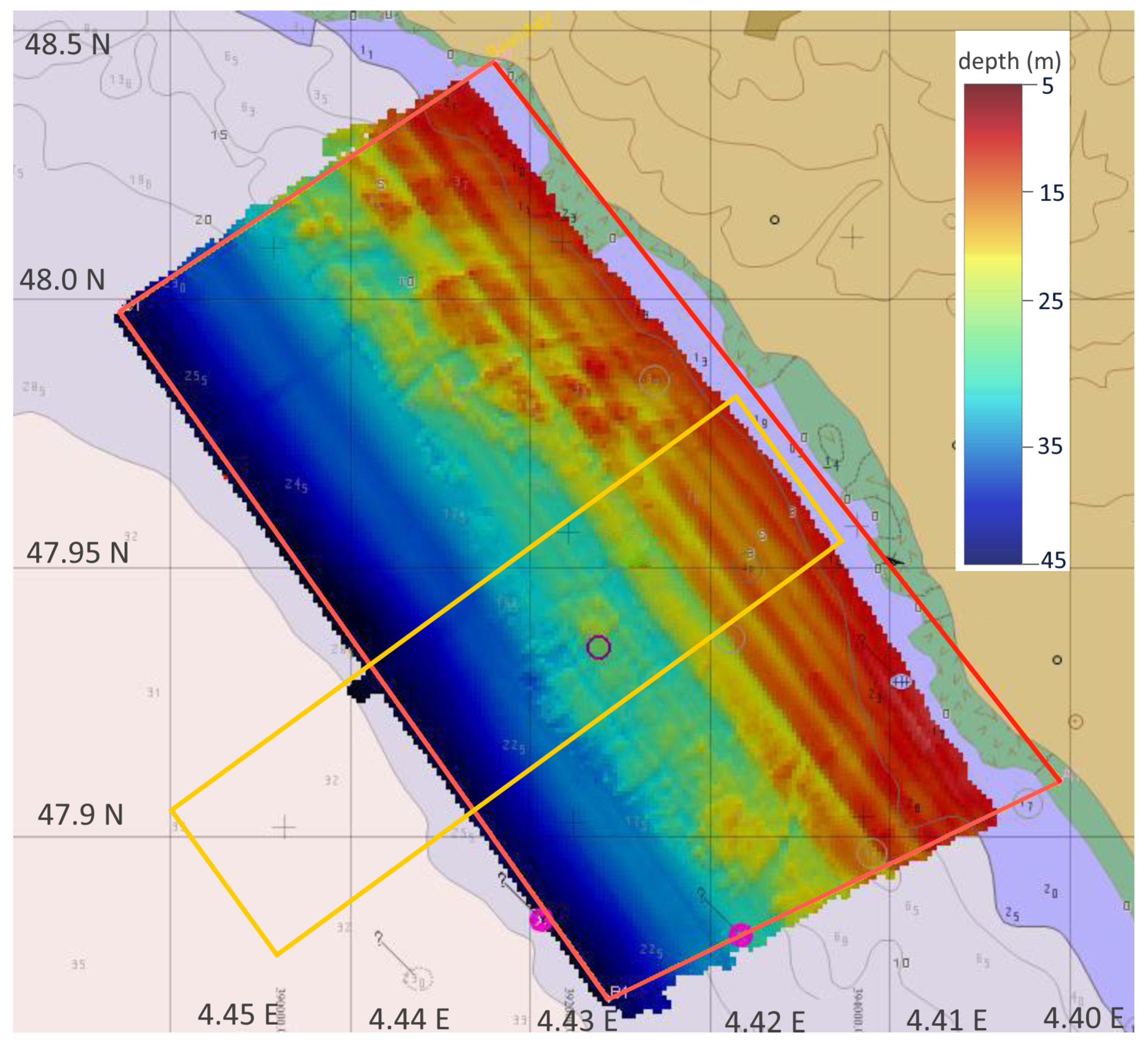
1.2. Site Bathymetry and Approximation
1.3. Analysis of the Wave Climate at the Investigation Site
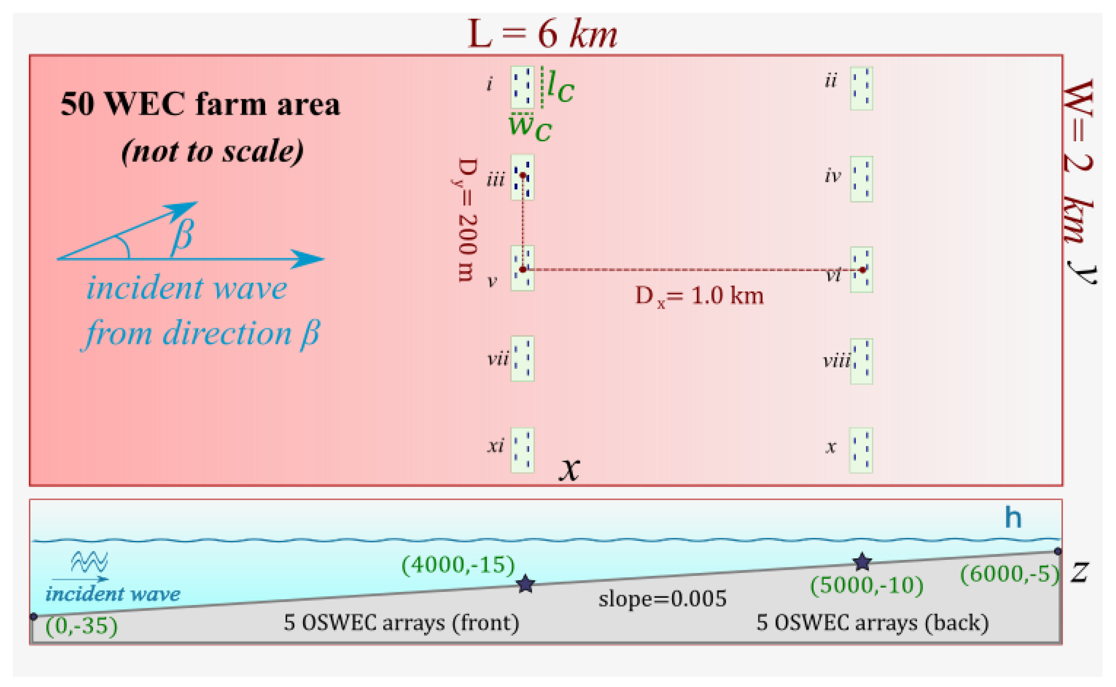
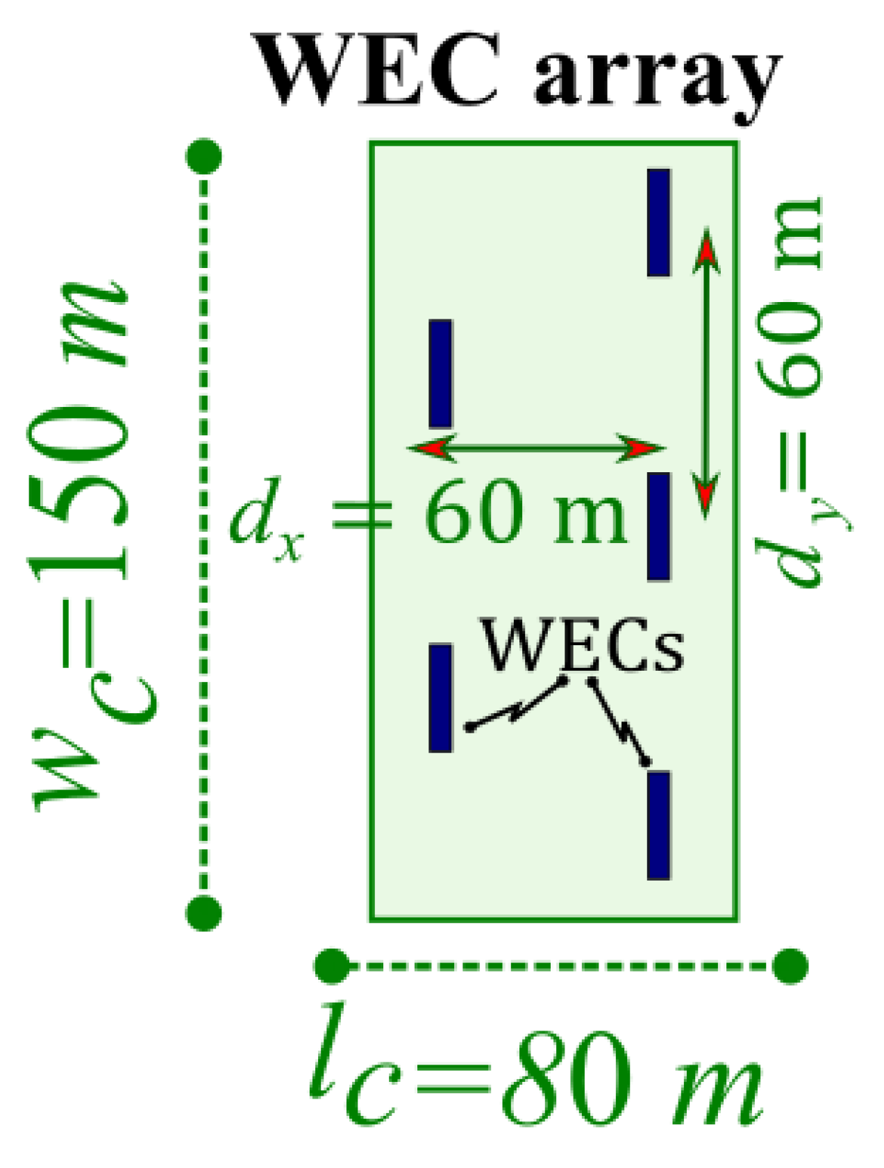
1.4. WEC Farm and Clustered WEC Array Layout
2. Wave-to-Wire Model Methodology
2.1. Modelled Scenarios
2.2. NEMOH BEM Model Parameters
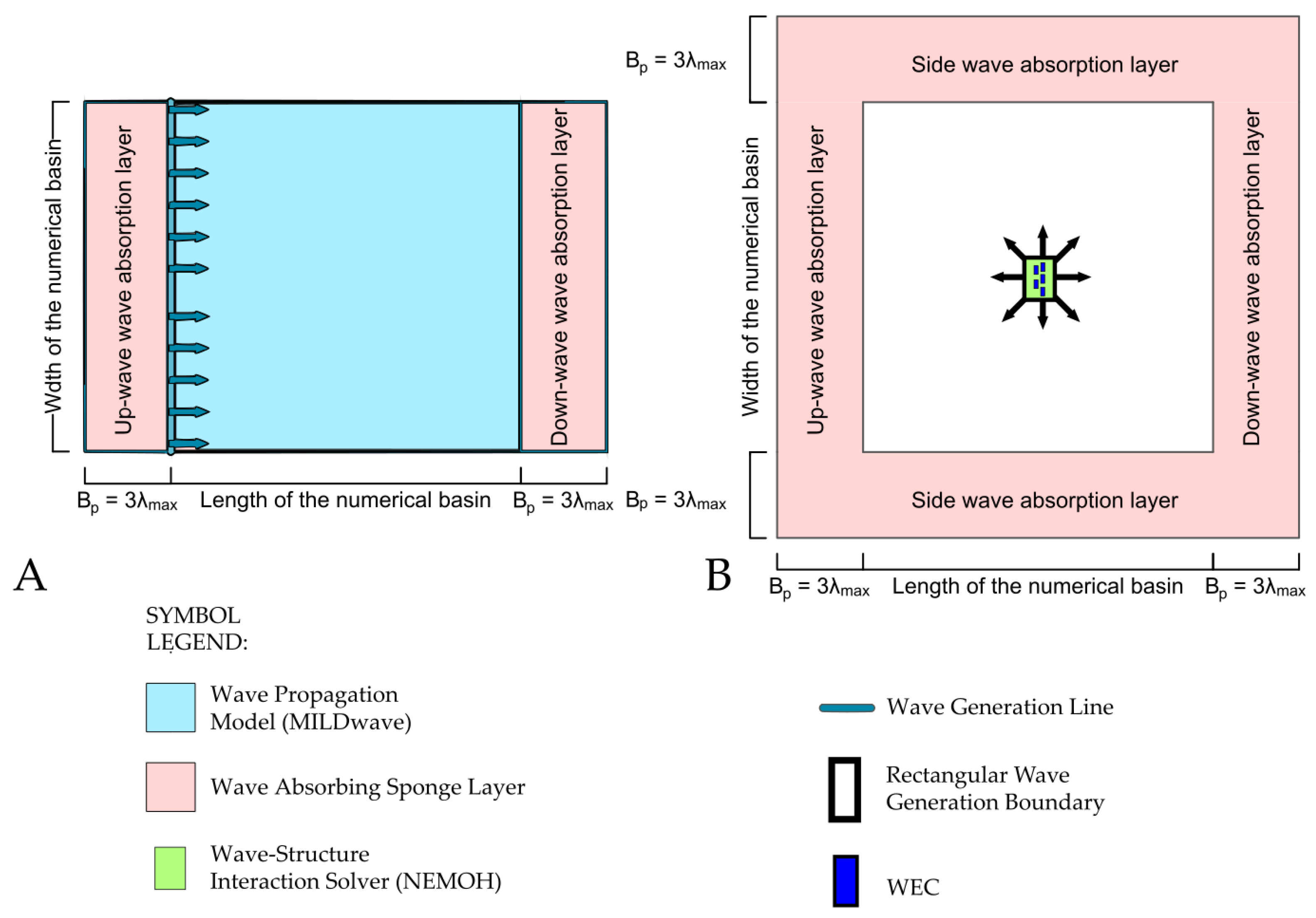
2.3. MILDwave Wave Propagation Model Parameters
2.4. Coupling of NEMOH to MILDwave
2.5. Simulating Irregular Sea States
2.6. Modelled OSWECs
2.7. Hydraulic PTO System and Derivation of the Optimal Coefficients for Irregular Waves
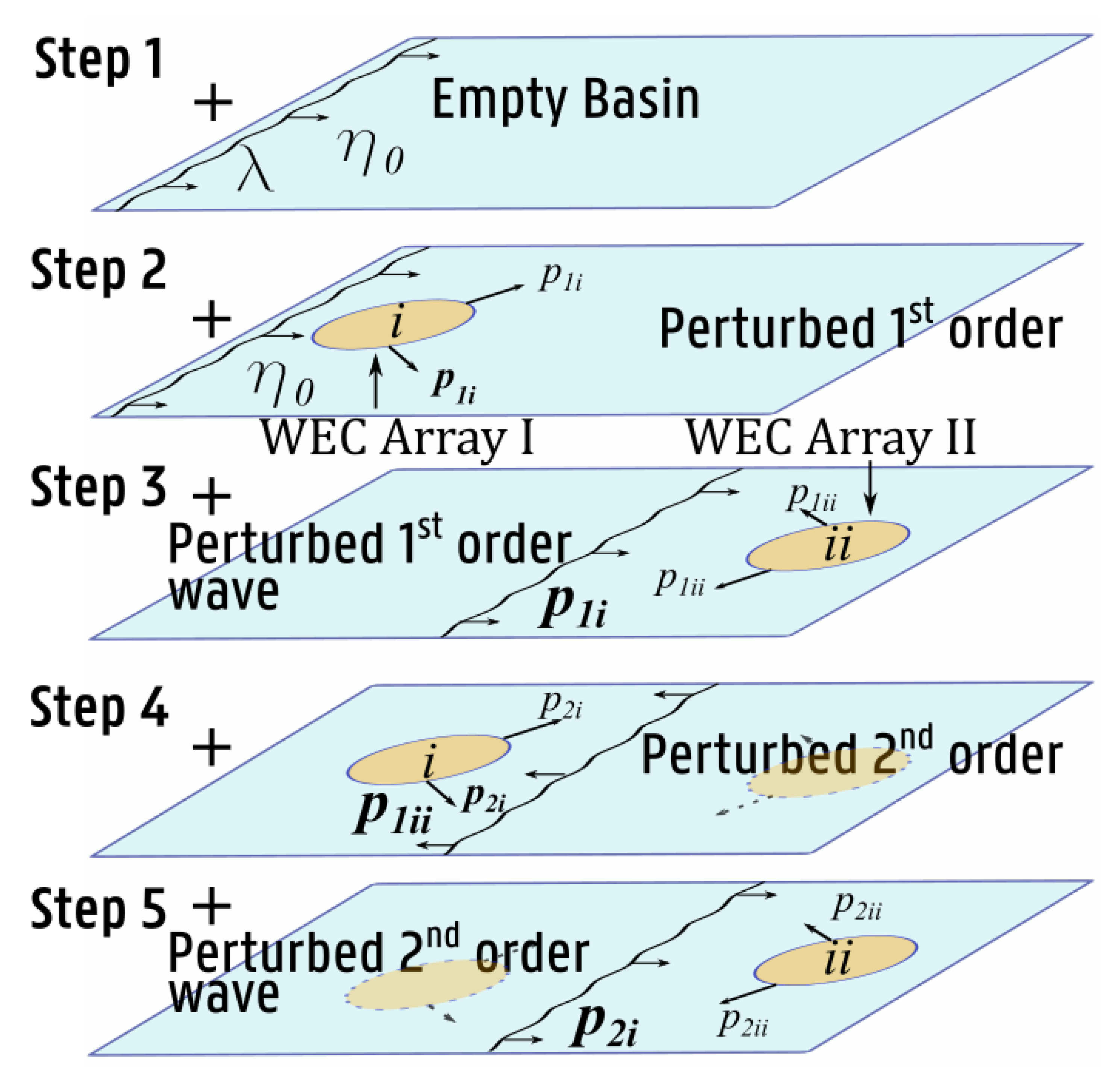
2.8. Calculating the Total Wave Field in the WEC Farm
3. Calculating the Power Output of a WEC Farm Composed of Multiple WEC Arrays
- the wave field inside each WEC array is computed in NEMOH using Equation (2),
- the power of each WEC in the array is calculated in WEC-Sim using the amplitudes output by NEMOH and summed for the WECs,
- the average perturbed 1st order wave field of the W2W model is computed at the WEC array perimeter,
- the power of the WEC array is multiplied by the wave field computed in the previous step,
- the power of the WEC farm is then the sum of the power of all constituent WEC arrays.
4. Results for a 2-Array 10 OSWEC Farm
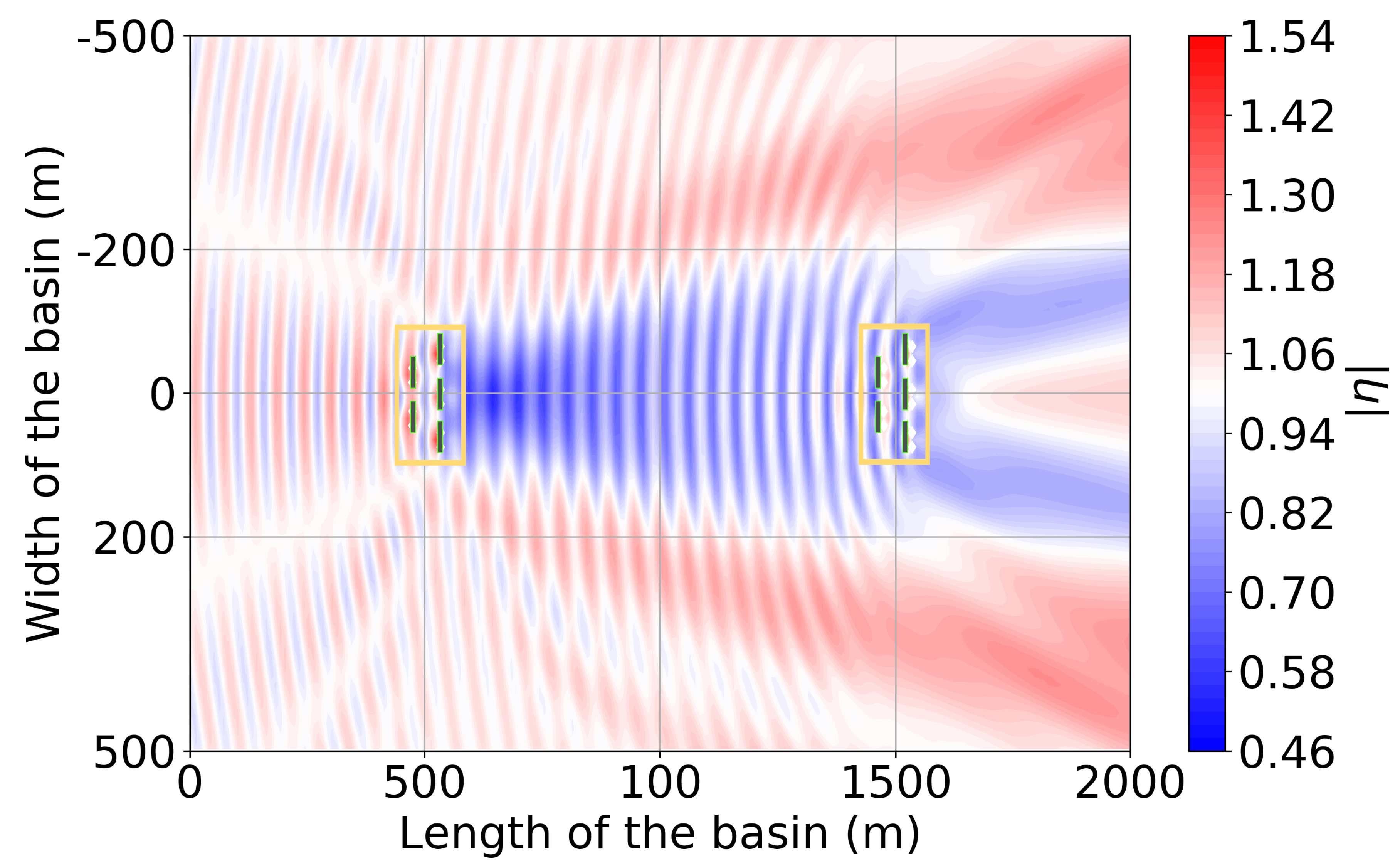
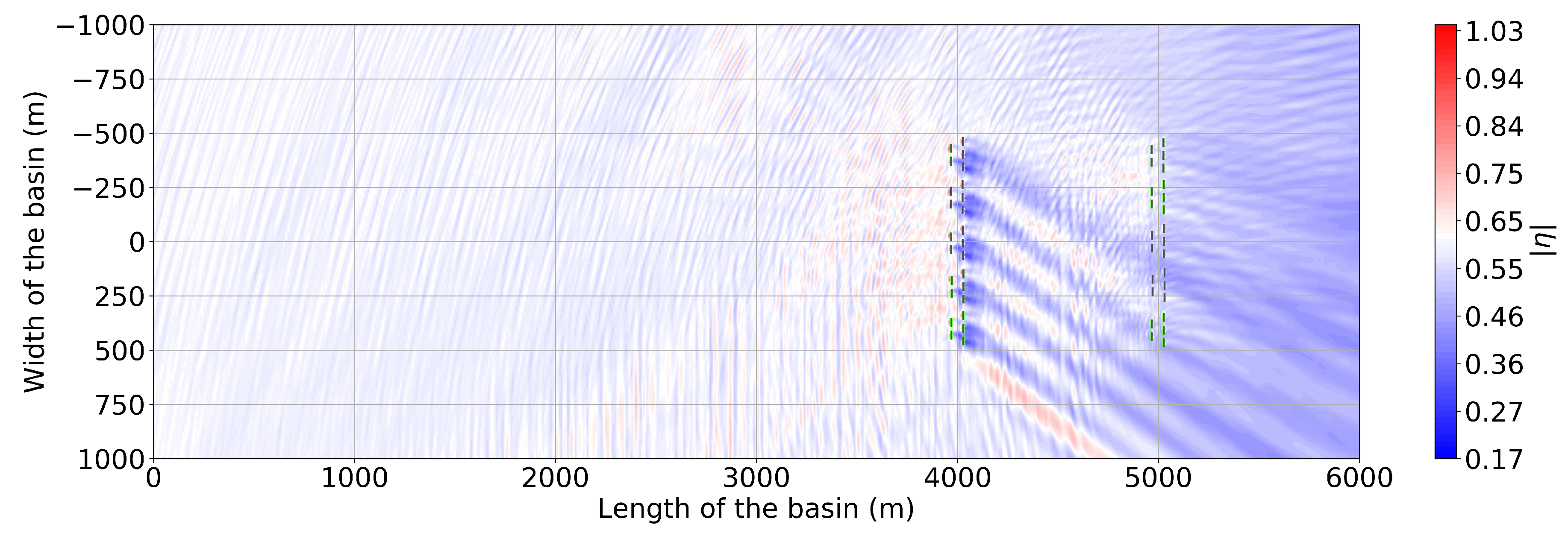
4.1. The 10-OSWEC Farm Wave Field for a Regular Wave at = 0 Incidence
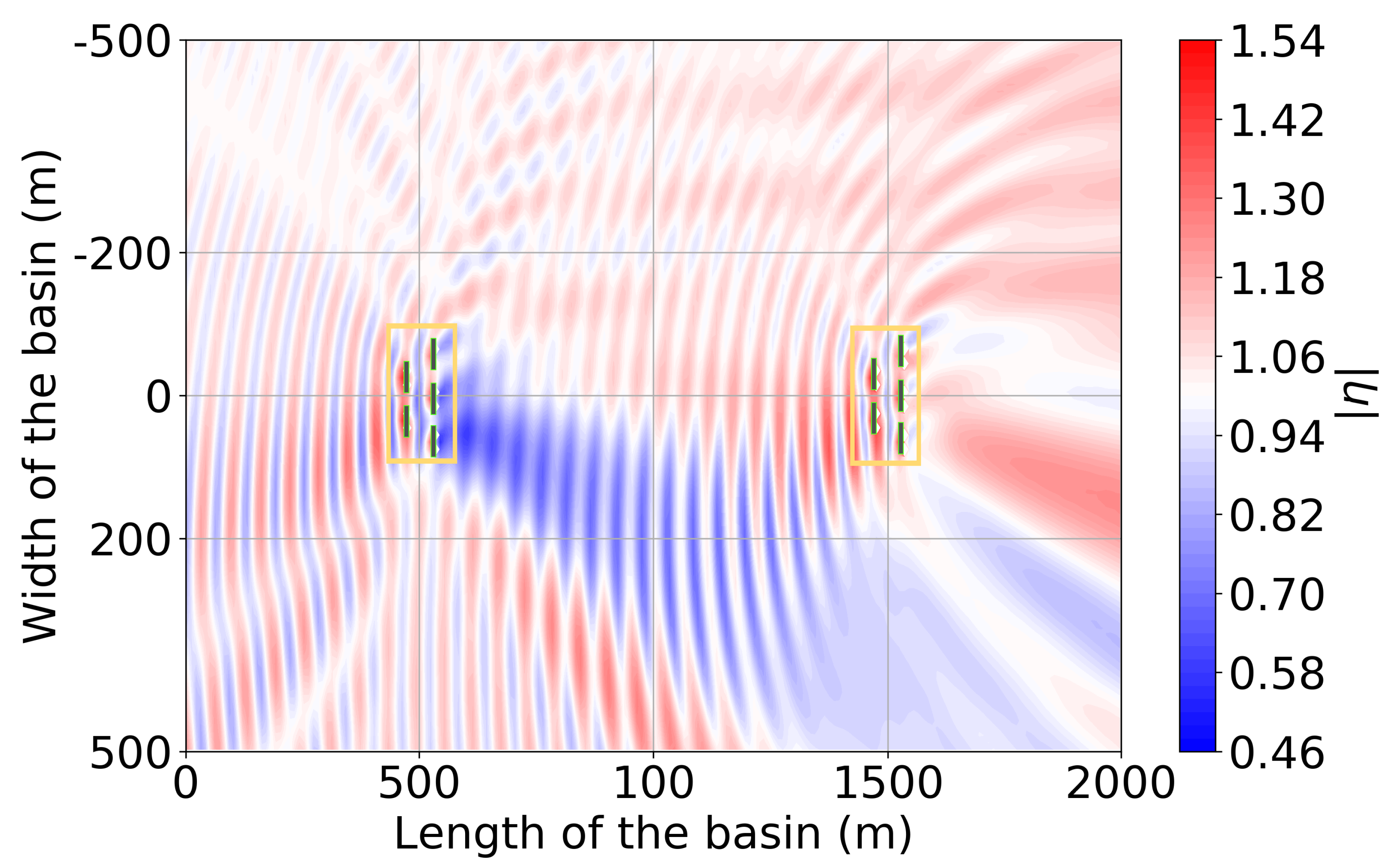
4.2. The 10-OSWEC Farm Wave Field for a Regular Wave at = 24 Incidence
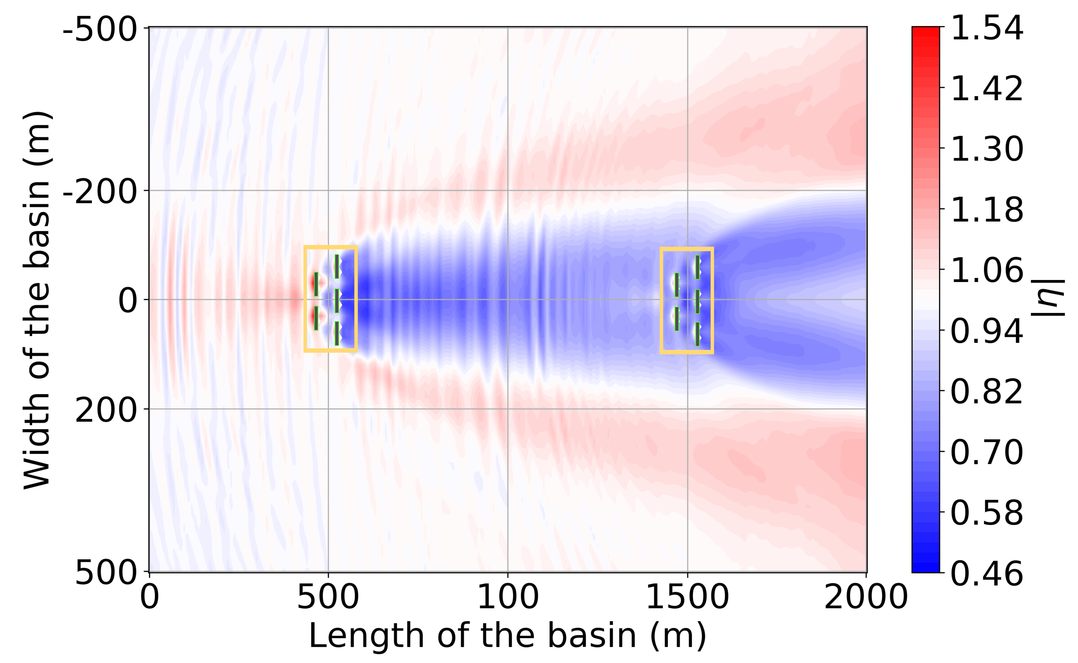
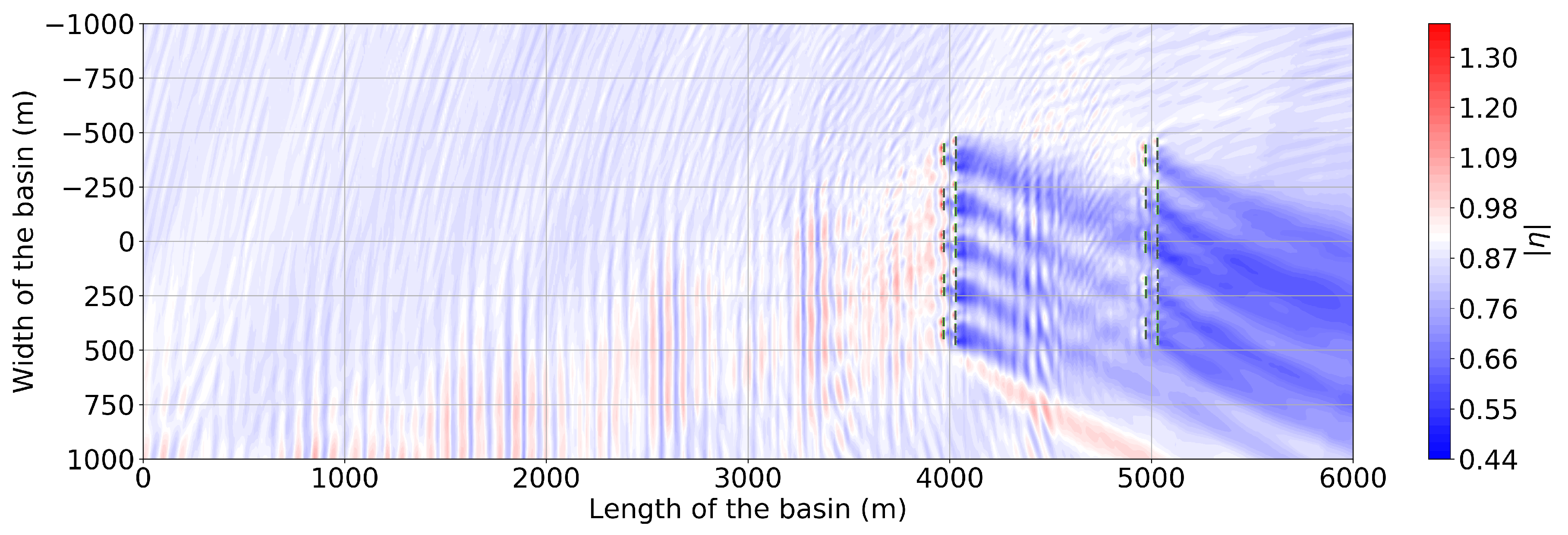
4.3. The 10-OSWEC Farm Wave Field for an Irregular Wave at = 0 Incidence
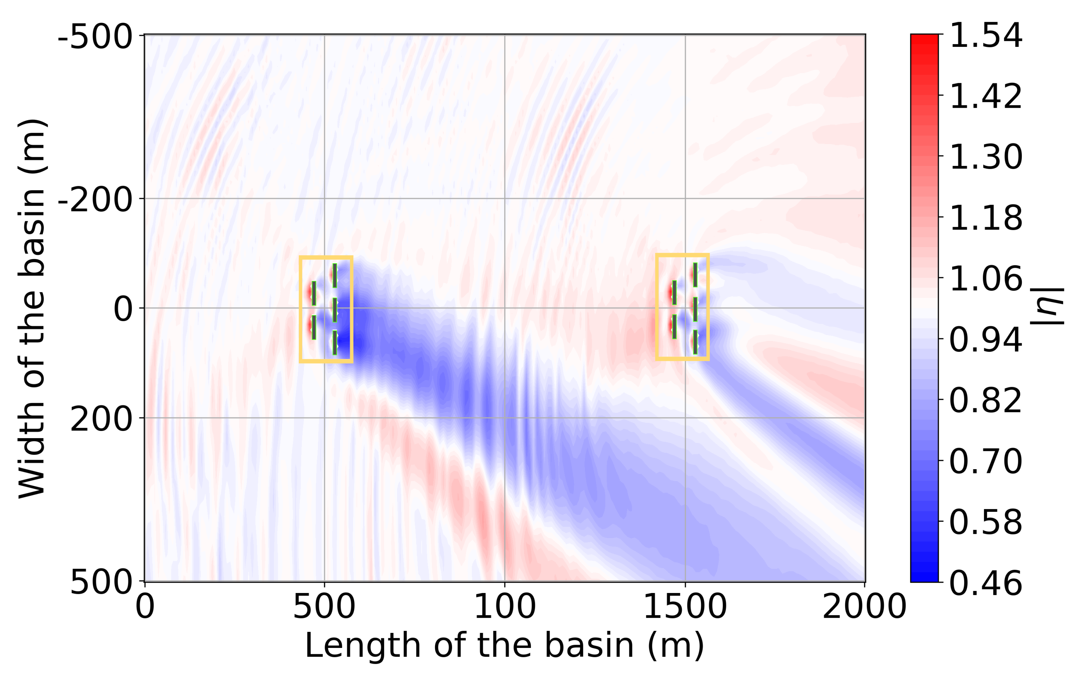
4.4. The 10-OSWEC Farm for an Irregular Wave at = 24 Incidence
5. Results for a 10 Array 50 OSWEC Farm
5.1. The 50-OSWEC Farm Wave Field for the Site Winter Climate
5.2. The 50-OSWEC Farm Wave Field for the Site Summer Climate
5.3. The 50-OSWEC Farm Wave Field for the Autumn Wave Climate
5.4. The Power Output of a 10 Array 50 OSWEC Farm for the Seasonal Wave Climate
5.4.1. Absolute Power Output of the 50-WEC Farm
5.4.2. Relative Power Output of the 50-WEC Farm
6. Discussion
7. Conclusions
Author Contributions
Funding
Acknowledgments
Conflicts of Interest
Abbreviations
| BEM | Boundary Element Method |
| CANDHIS | Centre d’Archivage National des Données de Houle In Situ |
| DoF | Degree of Freedom |
| OSWEC | Oscillating Surge Wave Energy Converter |
| PTO | Power Take-Off |
| RAO | Response Amplitude Operator |
| WEC | Wave Energy Converter |
| WSI | Wave-Strucure Interaction |
| W2W | Wave-to-wire |
| added moment of inertia (kg·m) | |
| angle of incidence of the incoming wave to the x-axis () | |
| , | WEC–WEC separation distances in the x and y direction (m) |
| hydrodynamic damping (kg/s) | |
| power-take-off linear damping coefficient (kg/s) | |
| power-take-off hydraulic damping equivalent coefficient (kg/s) | |
| variable motor displacement (rev/s) | |
| power take-off linear stiffness coefficient () | |
| number of bodies in the WEC array | |
| number of WEC arrays in a WEC farm | |
| absolute value of the complex free surface elevation (m) | |
| PTO system-force for hydraulic PTO system | |
| perturbed wave of order j for array i (-) | |
| mechanical power produced by the WEC with a linear PTO system | |
| mechanical power produced by the WEC with a hydraulic PTO system | |
| total power output of a WEC farm as if it were composed of isolated WEC arrays (kW) | |
| total power output of a WEC array including the intra-array effects (kW) | |
| total power output of an WEC farm including array effects (kW) | |
| q | q-value, defined as ratio of power of the -WEC array to the power produced by the sum of isolated WECs |
| piston area (m) | |
| resonance or natural period of an oscillating body (s) | |
| PTO-torque for linear PTO system | |
| PTO-torque for hydraulic PTO system | |
| complex amplitude of heave displacement | |
| heave displacement in time domain (m) | |
| wavelength (m) | |
| complex amplitude of pitch angular displacement | |
| pitch angular displacement in time domain (rad) | |
| wave amplitude (m) | |
| wave angular frequency (rad/s) | |
| ‘array effects’ = the hydrodynamic effects of WECs in an array that produce | |
| a perturbation in the incident wave field | |
| ‘intra-array’ referring to effects between WECs inside an array | |
| ‘inter-array’ referring to effects between disparate WEC arrays inside a WEC farm | |
| ‘near-field’ referring to wave field modification effects in the general location of the WECs inside an array | |
| ‘far-field’ referring to wave field modification effects outside the immediate area of the WEC array(s) | |
| ‘perturbed wave’ = radiated + diffracted wave |
References
- Balitsky, P.; Verao Fernandez, G.; Stratigaki, V.; Troch, P. Assessment of the Power Output of a Two-Array Clustered WEC Farm Using a BEM Solver Coupling and a Wave-Propagation Model. Energies 2018, 11, 2907. [Google Scholar] [CrossRef]
- O’Sullivan, A.; Lightbody, G. Wave to Wire Power Maximisation from a Wave Energy Converter. In Proceedings of the 11th European Wave and Tidal Energy Conference, Nantes, France, 6–11 September 2015. [Google Scholar]
- Bailey, H.; Robertson, B.R.; Buckham, B.J. Wave-to-wire simulation of a floating oscillating water column wave energy converter. Ocean Eng. 2016, 125, 248–260. [Google Scholar] [CrossRef]
- Penalba, M.; Ringwood, J. The Impact of a High-Fidelity Wave-to-Wire Model in Control Parameter Optimisation and Power Production Assessment. In Proceedings of the 37th International Conference on Ocean, Offshore and Artic Engineering, Madrid, Spain, 17–22 June 2018. [Google Scholar]
- Penalba, M.; Ringwood, J.V. A reduced wave-to-wire model for controller design and power assessment of wave energy converters. In Proceedings of the 2018 RENEW Conference, Lisbon, Portugal, 8–10 October 2018. [Google Scholar]
- Kasanen, E. AW-Energy—Positive experiences of the Waveroller in Portugal and France. In Proceedings of the WavEC Annual Seminar and International B2B Meetings, Lisbon, Portugal, 15–17 November 2015. [Google Scholar]
- AW-Energy Oy. WaveRoller. Available online: https://aw-energy.com/waveroller/ (accessed on 20 April 2019).
- CEREMA Eau, mer et fleuves—ER/MMH. Centre d’Archivage National de Données de Houle In Situ. Available online: http://candhis.cetmef.developpement-durable.gouv.fr/ (accessed on 24 April 2019).
- Troch, P.; Stratigaki, V. Phase-Resolving Wave Propagation Array Models. In Numerical Modelling of Wave Energy Converters; Folley, M., Ed.; Elsevier: London, UK, 2016; Chapter 10; pp. 191–216. [Google Scholar]
- Fernández, G.V.; Stratigaki, V.; Troch, P. Irregular Wave Validation of a Coupling Methodology for Numerical Modelling of Near and Far Field Effects of Wave Energy Converter Arrays. Energies 2019, 12, 538. [Google Scholar] [CrossRef]
- Balitsky, P.; Quartier, N.; Verao Fernandez, G.; Stratigaki, V.; Troch, P. Analyzing the Near-Field Effects and the Power Production of an Array of Heaving Cylindrical WECs and OSWECs Using a Coupled Hydrodynamic-PTO Model. Energies 2018, 11, 3489. [Google Scholar] [CrossRef]
- Yu, Y.; Lawson, M.; Ruehl, K.; Michelen, C. Development and Demonstration of the WEC-Sim Wave Energy Converter Simulation Tool. In Proceedings of the 2nd Marine Energy Technology Symposium, METS 2014, Seattle, WA, USA, 15–17 April 2014. [Google Scholar]
- Child, B.; Venugopal, V. Interaction of waves with an array of floating wave energy devices. In Proceedings of the 7th European Wave and Tidal Energy Conference, Porto, Portugal, 11–13 September 2007. [Google Scholar]
- Charrayre, F.; Benoit, M.; Peyrard, C.; Babarit, A. Modélisation des interactions dans une ferme de systèmes houlomoteursavec prise en compte de la bathymétrie. In Proceedings of the 14èmes Journées de l’Hydrodynamique, Nantes, France, 18–20 November 2014. [Google Scholar]
- Stratigaki, V.; Troch, P.; Stallard, T.; Forehand, D.; Folley, M.; Vantorre, M.; Kofoed, J.P.; Babarit, A.; Benoit, M. Development of a point absorber wave energy converter for investigation of array wake effect in large scale experiments. In Proceedings of the International Conference of the Application of Physical Modeling to Port and Coastal Protection, Ghent, Belgium, 17–20 September 2012; Troch, P., Stratigaki, V., De Roo, S., Eds.; Ghent University: Ghent, Belgium, 2013; pp. 787–796. [Google Scholar]
- Stratigaki, V.; Troch, P.; Stallard, T.; Forehand, D.; Kofoed, J.; Folley, M.A.; Benoit, M.; Babarit, A.; Kirkegaard, J. Wave Basin Experiments with Large Wave Energy Converter Arrays to Study Interactions between the Converters and Effects on Other Users. Energies 2014, 7, 701–734. [Google Scholar] [CrossRef]
- Göteman, M.; Engström, J.; Eriksson, M.; Isberg, J. Optimizing wave energy parks with over 1000 interacting point-absorbers using an approximate analytical method. Int. J. Mar. Energy 2015, 10, 113–126. [Google Scholar] [CrossRef] [Green Version]
- Ruiz, P.M.; Ferri, F.; Kofoed, J.P. Experimental Validation of a Wave Energy Converter Array Hydrodynamics Tool. Sustainability 2017, 9, 115. [Google Scholar] [CrossRef]
- Ruiz, P.M.; Nava, V.; Topper, M.B.R.; Minguela, P.R.; Ferri, F.; Kofoed, J.P. Layout Optimisation of Wave Energy Converter Arrays. Energies 2017, 10, 1262. [Google Scholar] [CrossRef]
- Zhao, H.T.; Sun, Z.L.; Hao, C.L.; Shen, J.F. Numerical modeling on hydrodynamic performance of a bottom-hinged flap wave energy converter. China Ocean Eng. 2013, 27, 73–86. [Google Scholar] [CrossRef]
- Schmitt, P.; Asmuth, H.; Elsäßer, B. Optimising power take-off of an oscillating wave surge converter using high fidelity numerical simulations. Int. J. Mar. Energy 2016, 16, 196–208. [Google Scholar] [CrossRef] [Green Version]
- Henry, A.; Folley, M.; Whittaker, T. A conceptual model of the hydrodynamics of an oscillating wave surge converter. Renew. Energy 2018, 118, 965–972. [Google Scholar] [CrossRef]
- Paredes, G.M.; Eskilsson, C.; Palm, J.; Bergdahl, L.; Leite, L.M.; Taveira-Pinto, F. Experimental and Numerical Modelling of a Moored, Generic Floating Wave Energy Converter. In Proceedings of the 10th European Wave and Tidal Energy Conference, Aalborg, Denmark, 2–5 September 2013. [Google Scholar]
- Schmitt, P.; Elsaesser, B. On the use of OpenFOAM to model oscillating wave surge converters. Ocean Eng. 2015, 108, 98–104. [Google Scholar] [CrossRef] [Green Version]
- Devolder, B.; Rauwoens, P.; Troch, P. Numerical simulation of a single floating point absorber wave energy converter using OpenFOAM. In Proceedings of the 2nd International Conference on Renewable energies Offshore, Lisbon, Portugal, 24–26 October 2016; pp. 197–205. [Google Scholar]
- Verbrugghe, T.; Domínguez, J.M.; Crespo, A.J.; Altomare, C.; Stratigaki, V.; Troch, P.; Kortenhaus, A. Coupling methodology for smoothed particle hydrodynamics modelling of nonlinear wave–structure interactions. Coast. Eng. 2018, 138, 184–198. [Google Scholar] [CrossRef]
- Devolder, B.; Stratigaki, V.; Troch, P.; Rauwoens, P. CFD simulations of floating point absorber wave energy converter arrays subjected to regular waves. Energies 2018, 11, 641. [Google Scholar] [CrossRef]
- Bharath, A. Numerical Analysis of Arrays of Wave Energy Converters. Ph.D. Thesis, University of Tasmania, Tasmania, Australia, 2018. [Google Scholar]
- Penalba, M.; Davidson, J.; Windt, C.; Ringwood, J.V. A high-fidelity wave-to-wire simulation platform for wave energy converters: Coupled numerical wave tank and power take-off models. Appl. Energy 2018, 226, 655–669. [Google Scholar] [CrossRef] [Green Version]
- Cargo, C.J.; Plummer, A.R.; Hillis, A.J.; Schlotter, M. Determination of optimal parameters for a hydraulic power take-off unit of a wave energy converter in regular waves. Proc. Inst. Mech. Eng. Part A J. Power Energy 2012, 226, 98–111. [Google Scholar] [CrossRef]
- Cargo, C.; Hillis, A.; Plummer, A. Optimisation and control of a hydraulic power take-off unit for a wave energy converter in irregular waves. Proc. Inst. Mech. Eng. Part A J. Power Energy 2014, 228, 462–479. [Google Scholar] [CrossRef] [Green Version]
- Folley, M.; Whittaker, T. The control of wave energy converters using active bipolar damping. Proc. Inst. Mech. Eng. Part M J. Eng. Marit. Environ. 2009, 223, 479–487. [Google Scholar] [CrossRef]
- De O. Falcão, A.F. Phase control through load control of oscillating-body wave energy converters with hydraulic PTO system. Ocean Eng. 2008, 35, 358–366. [Google Scholar]
- So, R.; Casey, S.; Kanner, S.; Simmons, A.; Brekken, T.K.A. PTO-Sim: Development of a power take off modeling tool for ocean wave energy conversion. In Proceedings of the 2015 IEEE Power Energy Society General Meeting, Denver, CO, USA, 26–30 July 2015; pp. 1–5. [Google Scholar]
- Sell, N.; Plummer, A.; Hillis, A.; Chandel, D. Modelling and calibration of a direct drive hydraulic PTO. In Proceedings of the 12th European Wave and Tidal Energy Conference (EWTEC2017), Cork, Ireland, 27 August–2 September 2017. [Google Scholar]
- Yu, Y.H.; Tom, N.; Jenne, D. Numerical Analysis on Hydraulic Power Take-Off for Wave Energy Converter and Power Smoothing Methods. In Proceedings of the 37th International Conference on Ocean, Offshore and Artic Engineering, Madrid, Spain, 17–22 June 2018; p. V010T09A043. [Google Scholar]
- Bento, A.R.; Rusu, E.; Martinho, P.; Soares, C.G. Assessment of the changes induced by a wave energy farm in the nearshore wave conditions. Comput. Geosci. 2014, 71, 50–61. [Google Scholar] [CrossRef]
- Carballo, R.; Iglesias, G. Wave farm impact based on realistic wave-WEC interaction. Energy 2013, 51, 216–229. [Google Scholar] [CrossRef]
- Rusu, E.; Onea, F. Study on the influence of the distance to shore for a wave energy farm operating in the central part of the Portuguese nearshore. Energy Convers. Manag. 2016, 114, 209–223. [Google Scholar] [CrossRef]
- Babarit, A.; Delhommeau, G. Theoretical and numerical aspects of the open source BEM solver NEMOH. In Proceedings of the 11th European Wave and Tidal Energy Conference, Nantes, France, 6–11 September 2015. [Google Scholar]
- Stratigaki, V. Experimental study and Numerical Modelling of Intra-Array Interactions and Extra-Array Effects of Wave Energy Converter Arrays. Ph.D. Thesis, Ghent University, Ghent, Belgium, 2014. [Google Scholar]
- Balitsky, P.; Verao Fernandez, G.; Stratigaki, V.; Troch, P. Coupling methodology for modelling the near-field and far-field effects of a Wave Energy Converter. In Proceedings of the ASME 36th International Conference on Ocean, Offshore and Arctic Engineering (OMAE 2017), Trondheim, Norway, 25–30 June 2017. [Google Scholar]
- Verbrugghe, T.; Stratigaki, V.; Troch, P.; Rabussier, R.; Kortenhaus, A. A Comparison Study of a Generic Coupling Methodology for Modeling Wake Effects of Wave Energy Converter Arrays. Energies 2017, 10, 1697. [Google Scholar] [CrossRef]
- Stratigaki, V.; Troch, P.; Forehand, D. A Fundamental Coupling Methodology for Modelling Near-Field and Far-Field Wave Effects of Floating Structures and Wave Energy Devices. Renew. Energy 2019. accepted. [Google Scholar]
- Beels, C.; Troch, P.; Backer, G.D.; Vantorre, M.; Rouck, J.D. Numerical implementation and sensitivity analysis of a wave energy converter in a time-dependent mild-slope equation model. Coast. Eng. 2010, 57, 471–492. [Google Scholar] [CrossRef]
- Babarit, A. On the park effect in arrays of oscillating wave energy converters. Renew. Energy 2013, 58, 68–78. [Google Scholar] [CrossRef] [Green Version]
- Penalba, M.; Touzón, I.; Lopez-Mendia, J.; Nava, V. A numerical study on the hydrodynamic impact of device slenderness and array size in wave energy farms in realistic wave climates. Ocean Eng. 2017, 142, 224–232. [Google Scholar] [CrossRef] [Green Version]
- European Marine Energy Centre Ltd. European Marine Energy Centre. Available online: https://aw-energy.com/waveroller/ (accessed on 10 April 2019).
- Tay, Z.Y.; Venugopal, V. Hydrodynamic interactions of oscillating wave surge converters in an array under random sea state. Ocean Eng. 2017, 145, 382–394. [Google Scholar] [CrossRef] [Green Version]
- Child, B.; Cruz, J.; Livingstone, M. The Development of a Tool for Optimising of Arrays of Wave Energy Converters. In Proceedings of the 9th European Wave and Tidal Energy Conference, Southampton, UK, 5–9 September 2011. [Google Scholar]
- Tomey-Bozo, N.; Babarit, A.; Murphy, J.; Stratigaki, V.; Troch, P.; Lewis, T.; Thomas, G. Wake effect assessment of a flap type wave energy converter farm under realistic environmental conditions by using a numerical coupling methodology. Coast. Eng. 2019, 143, 96–112. [Google Scholar] [CrossRef]
- Tomey-Bozo, N.; Murphy, J.; Lewis, T.; Troch, P.; Thomas, G. Flap type wave energy converter modelling into a time-dependent mild-slope equation model. In Proceedings of the 2nd International Conference on Offshore Renewable Energies, Glasgow, UK, 12–14 September 2016; pp. 277–284. [Google Scholar]
- Penalba, M.; Kelly, T.; Ringwood, J.V. Using NEMOH for modelling wave energy converters: A comparative study with WAMIT. In Proceedings of the 12th European Wave and Tidal Energy Conference (EWTEC2017), Cork, Ireland, 27 August–2 September 2017; pp. 631.1–631.10. [Google Scholar]
- Flavià, F.F.; McNatt, C.; Rongère, F.; Babarit, A.; Clément, A. A numerical tool for the frequency domain simulation of large arrays of identical floating bodies in waves. Ocean Eng. 2018, 148, 299–311. [Google Scholar] [CrossRef] [Green Version]
- Verao Fernandez, G.; Balitsky, P.; Stratigaki, V.; Troch, P. Coupling Methodology for Studying the Far Field Effects of Wave Energy Converter Arrays over a Varying Bathymetry. Energies 2018, 11, 2899. [Google Scholar] [CrossRef]
- Troch, P. MILDwave—A Numerical Model for Propagation and Transformation of Linear Water Waves; Technical Report; Internal Report; Department of Civil Engineering, Ghent University: Ghent, Belgium, 1998. [Google Scholar]
- Radder, A.; Dingemans, M. Canonical equations for almost periodic, weakly nonlinear gravity waves. Wave Motion 1985, 7, 473–485. [Google Scholar] [CrossRef]
- Vasarmidis, P.; Stratigaki, V.; Troch, P. Accurate and Fast Generation of Irregular Short Crested Waves by Using Periodic Boundaries in a Mild-Slope Wave Model. Energies 2019, 12, 785. [Google Scholar] [CrossRef]
- Pastor, J.; Liu, Y. Frequency and time domain modeling and power output for a heaving point absorber wave energy converter. Int. J. Energy Environ. Eng. 2014, 5, 101. [Google Scholar] [CrossRef]
- Child, B.; Venugopal, V. Optimal Configurations of wave energy devices. Ocean Eng. 2010, 37, 1402–1417. [Google Scholar] [CrossRef]
- De Andrés, A.; Guanche, R.; Meneses, L.; Vidal, C.; Losada, I. Factors that influence array layout on wave energy farms. Ocean Eng. 2014, 82, 32–41. [Google Scholar] [CrossRef]
- Sharp, C.; DuPont, B.A. Multi-Objective Real-Coded Genetic Algorithm Method for Wave Energy Converter Array Optimization. In Proceedings of the ASME International Conference on Offshore Mechanics and Arctic Engineering, Busan, Korea, 19–24 June 2016; Volume 6. [Google Scholar]
- McNatt, J.C.; Venugopal, V.; Forehand, D. A novel method for deriving the diffraction transfer matrix and its application to multi-body interactions in water waves. Ocean Eng. 2015, 94, 173–185. [Google Scholar] [CrossRef]
- Rijnsdorp, D.; Hansen, J.; Lowe, R. Predicting coastal impacts of wave farms using a wave-resolving model. In Proceedings of the 12th European Wave and Tidal Energy Conference (EWTEC2017), Cork, Ireland, 27 August–2 September 2017. [Google Scholar]


| Winter | Spring | Summer | Autumn | Year | |
|---|---|---|---|---|---|
| (m) | 2.55 | 1.75 | 1.20 | 1.80 | 1.87 |
| (s) | 11.71 | 10.45 | 8.71 | 10.54 | 10.34 |
| 261.74 | 263.32 | 270.12 | 263.16 | 264.48 |
| Wave Height H (m) | Wave Period T (s) | Wave Incidence Angle |
|---|---|---|
| 2.0 | 10.0 | 0 |
| 2.0 | 10.0 | 20 |
| Simulated Case | Winter | Summer | Autumn |
|---|---|---|---|
| (m) | 2.55 | 1.20 | 1.80 |
| (s) | 11.71 | 8.71 | 10.54 |
| () | −20.0 | −30.0 | −22.0 |
| wave peak period | (s) | 8.71 | 10.54 | 11.71 |
| hydraulic PTO damping coefficient | 198.7 | 145.6 | 121 |
| Array i Array vi | Array ii Array vii | Array iii Array viii | Array iv Array ix | Array v Array x | Total Power per Row [kW] | Total Power [kW] |
|---|---|---|---|---|---|---|
| 743.13 | 774.77 | 772.83 | 744.26 | 733.79 | 3768.78 | |
| 771.63 | 620.77 | 546.93 | 585.96 | 567.38 | 3092.67 | 6861.45 |
| Array i Array vi | Array ii Array vii | Array iii Array viii | Array iv Array ix | Array v Array x | Total Power per Row [kW] | Total Power [kW] |
|---|---|---|---|---|---|---|
| 607.14 | 629.09 | 615.59 | 621.04 | 603.41 | 3076.27 | |
| 595.74 | 595.26 | 489.20 | 490.51 | 484.22 | 2654.93 | 5731.20 |
| Array i Array vi | Array ii Array vii | Array iii Array viii | Array iv Array ix | Array v Array x | Total Power per Row [kW] | Total Power [kW] |
|---|---|---|---|---|---|---|
| 686.76 | 699.57 | 705.83 | 708.32 | 698.83 | 3499.30 | |
| 699.34 | 592.99 | 498.44 | 561.49 | 546.08 | 2898.34 | 6397.64 |
| Array i Array vi | Array ii Array vii | Array iii Array viii | Array iv Array ix | Array v Array x | Average q-Value per Row | Average q-Value Farm |
|---|---|---|---|---|---|---|
| 0.93 | 0.97 | 0.97 | 0.93 | 0.92 | 0.95 | |
| 0.97 | 0.78 | 0.69 | 0.74 | 0.72 | 0.78 | 0.86 |
| Array i Array vi | Array ii Array vii | Array iii Array viii | Array iv Array ix | Array v Array x | Average q-Value per Row | Average q-Value Farm |
|---|---|---|---|---|---|---|
| 0.99 | 1.03 | 1.00 | 1.01 | 0.98 | 1.00 | |
| 0.97 | 0.97 | 0.80 | 0.80 | 0.79 | 0.87 | 0.93 |
| Array i Array vi | Array ii Array vii | Array iii Array viii | Array iv Array ix | Array v Array x | Average q-Value per Row | Average q-Value Farm |
|---|---|---|---|---|---|---|
| 0.91 | 0.93 | 0.94 | 0.94 | 0.93 | 0.93 | |
| 0.93 | 0.79 | 0.66 | 0.75 | 0.73 | 0.77 | 0.85 |
© 2019 by the authors. Licensee MDPI, Basel, Switzerland. This article is an open access article distributed under the terms and conditions of the Creative Commons Attribution (CC BY) license (http://creativecommons.org/licenses/by/4.0/).
Share and Cite
Balitsky, P.; Quartier, N.; Stratigaki, V.; Verao Fernandez, G.; Vasarmidis, P.; Troch, P. Analysing the Near-Field Effects and the Power Production of Near-Shore WEC Array Using a New Wave-to-Wire Model. Water 2019, 11, 1137. https://doi.org/10.3390/w11061137
Balitsky P, Quartier N, Stratigaki V, Verao Fernandez G, Vasarmidis P, Troch P. Analysing the Near-Field Effects and the Power Production of Near-Shore WEC Array Using a New Wave-to-Wire Model. Water. 2019; 11(6):1137. https://doi.org/10.3390/w11061137
Chicago/Turabian StyleBalitsky, Philip, Nicolas Quartier, Vasiliki Stratigaki, Gael Verao Fernandez, Panagiotis Vasarmidis, and Peter Troch. 2019. "Analysing the Near-Field Effects and the Power Production of Near-Shore WEC Array Using a New Wave-to-Wire Model" Water 11, no. 6: 1137. https://doi.org/10.3390/w11061137