Spatial Pattern Analysis and Prediction of Gully Erosion Using Novel Hybrid Model of Entropy-Weight of Evidence

Abstract

Gully erosion is an environmental problem in arid and semi-arid areas. Gullies threaten the soil and water resources and cause off- and on-site problems. In this research, a new hybrid model combines the index-of-entropy (IoE) model with the weight-of-evidence (WoE) model. Remote sensing and GIS techniques are used to map gully-erosion susceptibility in the watershed of the Bastam district of Semnan Province in northern Iran. The performance of the hybrid model is assessed by comparing the results with from models that use only IoE or WoE. Three hundred and three gullies were mapped in the study area and were randomly classified into two groups for training (70% or 212 gullies) and validation (30% or 91 gullies). Eighteen topographical, hydrological, geological, and environmental conditioning factors were considered in the modeling process. Prediction-rate curves (PRCs) and success-rate curves (SRCs) were used for validation. Results from the IoE model indicate that drainage density, slope, and rainfall factors are the most important factors promoting gullying in the study area. Validation results indicate that the ensemble model performed better than either the IoE or WoE models. The hybrid model predicted that 38.02 percent of the study area has either high or very high susceptible to gullying. Given the high accuracy of the novel hybrid model, this scientific methodology may be very useful for land use management decisions and for land use planning in gully-prone regions. Our research contributes to achieve Land Degradation Neutrality as will help to design remediation programs to control non-sustainable soil erosion rates.

1. Introduction

Soil erosion in arid and semi-arid regions is one of the important factors that should be taken into consideration in land use planning [1,2,3]. Soil erosion is a major consequence of environmental and ecological change [4,5,6]. Water soil erosion has long been of interest to soil conservation researchers [1]. Topography, types of landforms, and resistance to erosion are the main determinants of erosion type and severity, and this is especially the case with linear erosion processes such as gullies [7].

Among the types of erosion, gully erosion most threatens numerous environmental resources and land use sustainability. This threat is not limited to soil degradation, changes in the landscape and/or landcover, limitations of agricultural activities, or the economic exploitation of natural resources. Gully erosion also promotes the initiation and expansion of badlands, promotes floods, lowering of water tables, desertification, and production and transportation of significant volumes of sediments along the watersheds to the coastal and lowlands [8,9,10].

A gully is a drainage channel with steeply sloping sidewalls and an active, steep eroding head-cut caused by fluctuating surface flows (i.e., during or after severe rainfall) [11]. Most scholars regard the destruction of natural ecosystems, non-sustainable land uses, degradation of vegetative cover, overgrazing, climate change, geological conditions, and human disturbance of natural systems to be the main causes of gullying [12,13,14,15,16,17,18,19].

Some studies have found that the range of sediment production attributable to gully erosion is 10% to 94% in different ecosystems and that spatial and temporal factors, soil types, land uses, topography, climate, and others can also influence sediment production [11]. A study of 22 watersheds in Spain determined that annual sediment production in areas without gullying is 0.74 Mg/ha, but in similar environments where gullying is occurring the annual production is 2.97 Mg/ha [20]. A single gully can generate sediments annually at a rate of up to 93,750 Mg/km [21].

Because the erosion is so fast at the head of a gully, there are no measures that can be taken to control or stop head-cut development; the measures that are taken are likely to only slow down their growth [22]. To prevent the rapid growth of gullies or to minimize the damage they cause, it is vital to understand the morphology of a gully, the manner in which it forms, and the causes for its development. Studying the amount of development of gully head-cut erosion in a specific timeframe can enable the prediction of the rate of expansion and growth, and this can also improve damage estimates. Identification of areas that are more susceptible to gully erosion is therefore possible. Accurate and adequate information about the type and extent of headward head-cut erosion can enable better land use decisions and more effective environmental management [23].

For more than a half-century, prediction and modeling of soil erosion have been a valuable component of soil conservation and engineering planning [24]. Mathematical simulations can be used to estimate erosion that is caused by an array of independent factors. Geomorphologic models are empirically based and must not include theoretical assumptions of relationships. They also must avoid scenarios and should not ignore multicollinearity among conditioning factors for the phenomenon [25]. Without a clear explanation of a geomorphological conceptual model, it is impossible to identify the appropriate sub-models that can numerically express the phenomenon [25]. The solution is to define the modeling goals and to identify the unknowns about the phenomenon; only then can a conceptual model for the desired phenomenon be developed, tested, and validated [26]. Modeling of soil erosion requires many empirical measurements of a landscape. Remote sensing techniques that produce aerial photographs, satellite data, or radar data, have eased the difficulty of this otherwise laborious problem [27].

In the last decades, several gully-erosion models have been developed to aid gully- erosion susceptibility mapping (GESM). These models can be classified into three groups: knowledge based models like the analytic hierarchy process (AHP) [16]; bivariate and multivariate statistical models like conditional probability (CP) [28], information value (IV) [29], frequency ratio (FR) [13], index of entropy (IoE) [30], evidential belief function (EBF) [14], weights-of-evidence (WOE) [31], certainty factor (CF) [32], and logistic regression (LR) [33]; and machine-learning models like maximum entropy (ME) [19], multivariate adaptive regression spline (MARS) [15], artificial neural network (ANN) [34], boosted regression tree (BRT) [35], linear discriminant analysis (ADA) [17], bagging best-first decision tree (Bag-BFTree) [36], random forest (RF) [37], flexible discriminant analysis (FDA) [38], support vector machine (SVM) [39], and classification and regression trees (CART) [15].

Each model has disadvantages and advantages. Therefore, improve performance of gully-erosion models; this study uses a hybrid approach to identify gully-erosion susceptible areas. A region that is heavily impacted by gully erosion is the Bastam district watershed in Semnan Province, of northern Iran. Gully erosion occurs in this area due to the highly erodible soils of these lands and misuse of soil and water resources. This has led to the destruction and transformation of agricultural lands into wastelands, the destruction of communication infrastructure, and damage to residential areas. In this study, two models of WoE and IoE are combined to map gully-erosion susceptibility in the Bastam district watershed. These two models have been previously used in studies of other fields of destructive geomorphological and hydrological phenomena, such as landslides [40,41,42], floods [43], and groundwater depletion [44,45].

2. Materials and Methods

2.1. Study Area

The Bastam watershed covers a 1329 km² area (36°27′02″ to 36°47′13″ N, and 54°24′23″ to 55°11′08″ E (Figure 1). Elevation in the study area ranges from 1357 m a.s.l. to 3893 m a.s.l. The mean elevation is 278.34 m a.s.l.). The minimum and maximum slopes are 0° and 70.66°; the mean is 13.55°. The central and south parts of the watershed have relatively smooth topography with gentle slopes. The rest of the study area is mountainous; is part of the Alborz Mountains. The watershed experiences a mean annual rainfall amount of 262 mm. The mean annual temperature is 12.8 °C [46]. More than 25% of the land is poor rangeland. Another 22.84% is covered by a relatively sparse forest, while 0.01% is covered in dense forest and 0.01% is land on which dryland-farming is practiced. The main lithographic units include high elevation piedmont fans and valley terrace deposits, stream channels, braided channels, floodplain deposits, and low elevation piedmont fans, and valley terrace deposits [47]. Rock outcrops, entisols, entisols/inceptisols, and mollisols are the most common geological and pedological surfaces in the study area [48]. Morphometric analysis of gullies in the study area shows that approximately 9.3% of the study area is affected by gully erosion. This indicates that the study area is very susceptible to gully erosion. There are more gullies in the south-central portion of the study area where slopes are lower than in the northern parts of the study area where slopes are steep and rocky outcrops are abundant and few gullies form. Gullies range in length from several meters to several hundred meters and their depths can be several meters. Gully width also varies, ranging from several centimeters to several meters. Gullies in the northern parts of the study area have V-shaped cross-sections, whereas in the central and southern parts of the region, due to more erodible soils, concentrated runoff because of low slope, and the more resistant sediments on the floor of the watershed prevent erosion, so the valleys are U-shaped.

2.2. Methodology

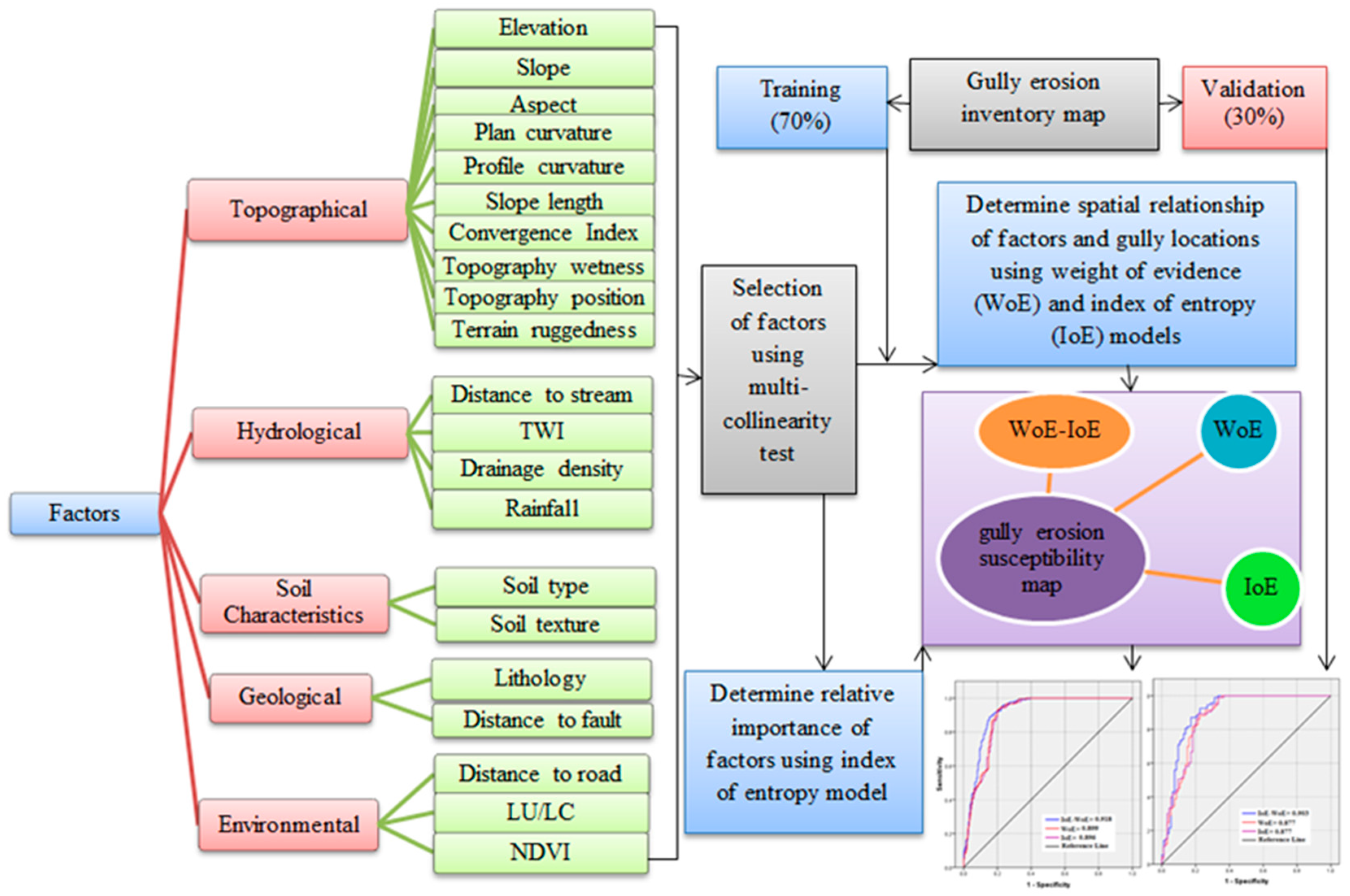
This study involved six steps (Figure 2): data preparation, including the creation of a GEIM, compilation of thematic layers depicting the spatial distribution of gully-erosion conditioning factors (GECFs), and division of GEIM into training and validation groups; multi-collinearity analyses of the GECFs using indices of tolerance (TOL) and variance inflation factor (VIF); application of the WoE model to analyze the spatial relationship between GECFs and gully locations; determination of the importance of the GECFs using the IoE model; preparation of the GESM using the WoE and IoE models separately; and integration of the hybrid WoE-IoE model; and validation using the area-under-the-curve receiver-operating characteristic (AUROC).

2.2.1. Gully-erosion Inventory Map (GEIM)

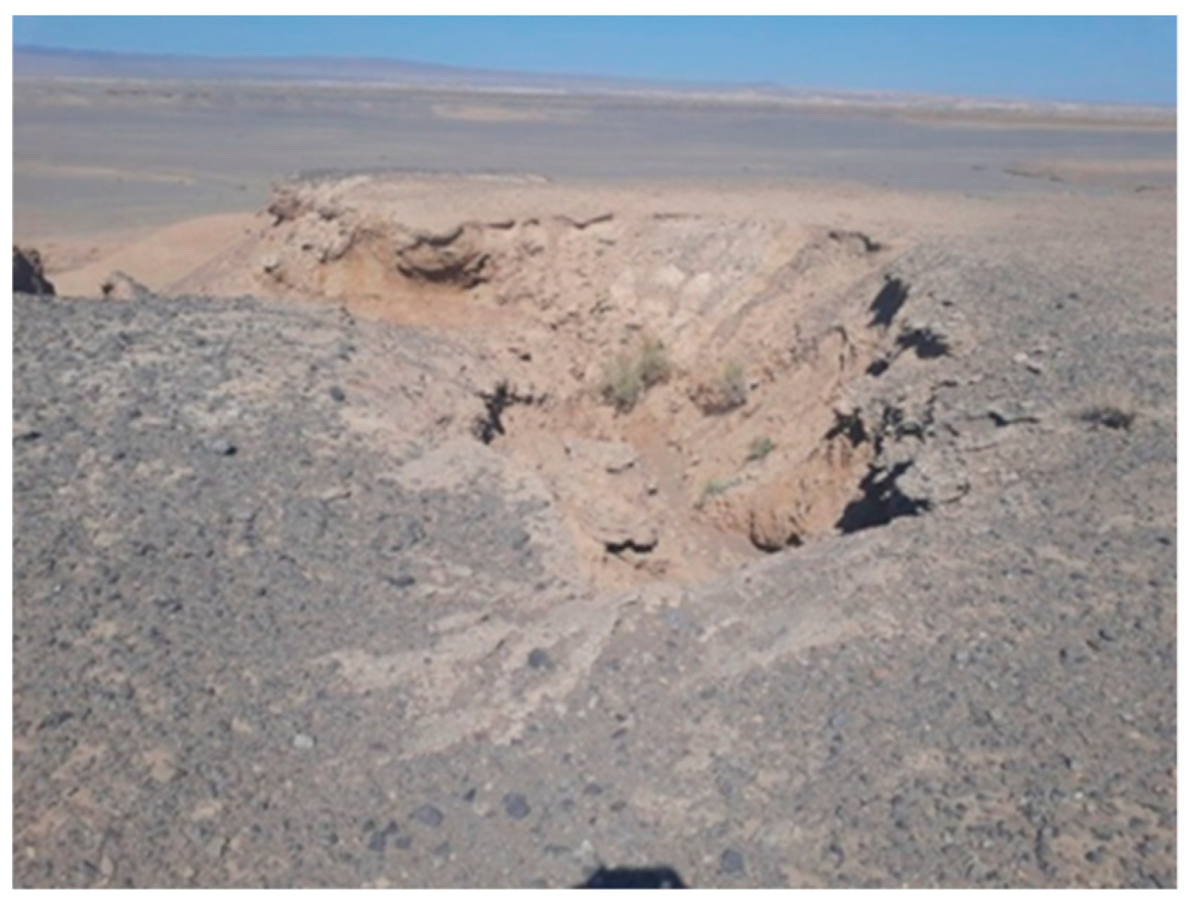
A GEIM shows the spatial distribution of gullies and this is necessary to determine the spatial distribution of susceptibility to gullying [15]. Data acquired from the Agricultural and Natural Resources Research Center of Semnan Province were combined with extensive field surveys (Figure 3) and interpretation of satellite imagery to map gully erosion in the study area. Three hundred and three gullies were identified in the study area (Figure 1) and this set was randomly separated into two groups for modeling (70% or 212 gullies) and validation (30% or 91 gullies). In addition, an equivalent number (303) of locations without gullies were randomly selected using the random-point tool in ArcGIS to support calibration and validation [49]. The maximum and minimum lengths of the 303 gullies are 346 m and 0.74 m, respectively, whereas, the maximum depth is 7.2 m and the minimum depth is 0.65 m. The maximum width is 16.6 m and the minimum width is 0.74 m.

2.2.2. Gully Erosion Conditioning Factors (GECFs)

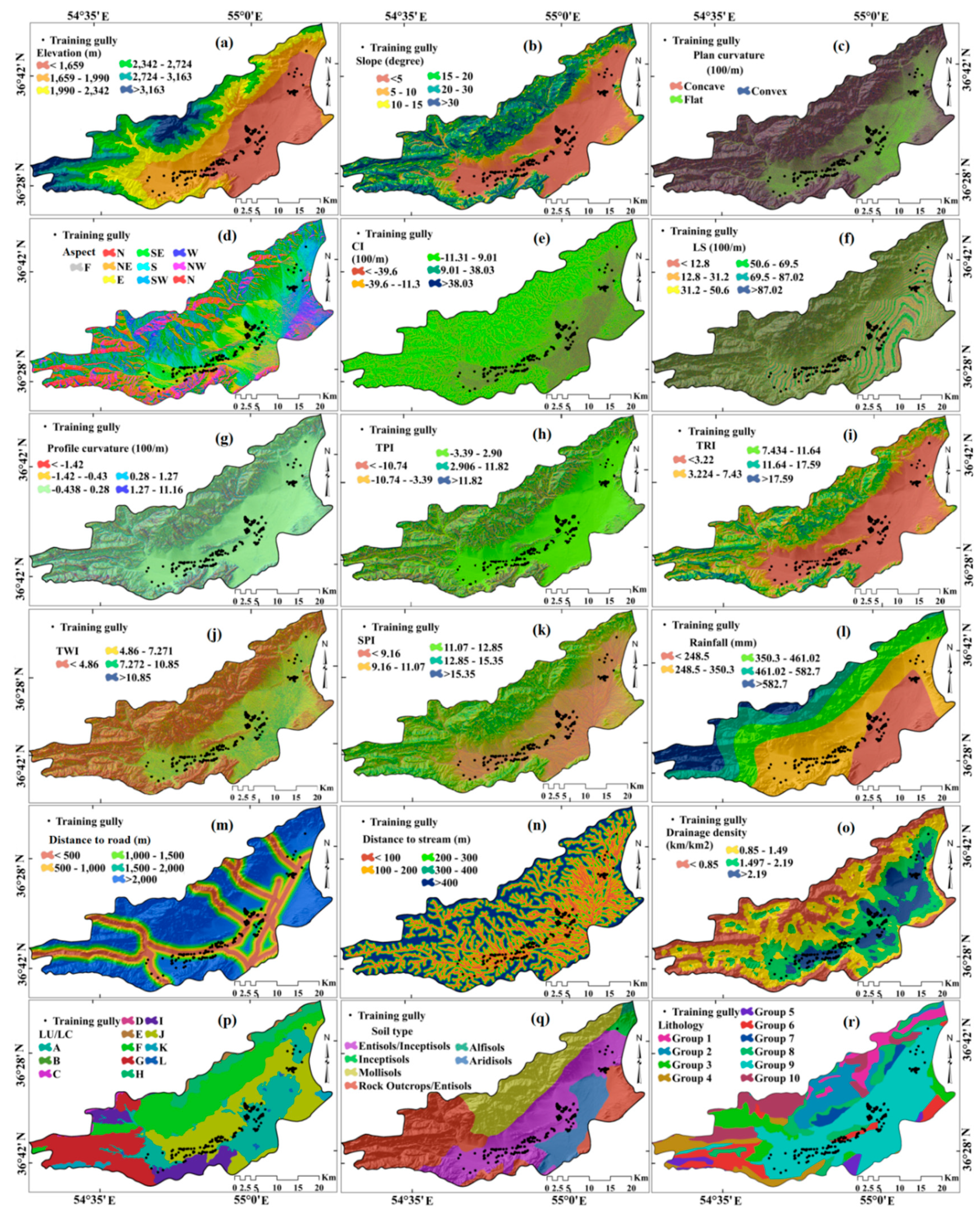
Gullying results from the interaction of several environmental factors that include hydrology, topography, land use/land cover, soil characteristics, human activities, and rainfall [50]. In this study, 18 GECFs were selected and mapped: elevation (m), slope (°), plan curvature (100/m), aspect, convergence index (100/m), slope length (LS), profile curvature (100/m), topography position index (TPI), terrain ruggedness index (TRI), topography wetness index (TWI), stream power index (SPI), rainfall (mm), distance to road (m), distance to stream (m), drainage density (km/km²), land use/land cover (LU/LC), soil type, and lithology (Figure 4a–r). These factors were obtained from several sources. The geological map at the scale of 1:100,000 and made by the Geological Society of Iran (GSI) (http://www.gsi.ir/) was used to produce the lithology map. Ten lithological units in the study area were created based upon formation and susceptibility to gully erosion (

Table 1. The lithology of the study area.

Group	Unit	Description	Age
1	Cm	Dark grey to black fossiliferous limestone with subordinate black shale ( MOBARAK FM )	Carboniferous
2	DCkh	Yellowish, thin to thick-bedded, fossileferous argillaceous limestone, dark grey limestone, greenish marl and shale, locally including gypsum	Devonian
3	Ea.bvs	Andesitic to basaltic volcano sediment	Eocene
	Ek	Well bedded green tuff and tuffaceous shale (KARAJ FM)	Eocene
	Ea.bv	Andesitic and basaltic volcanic	Eocene
4	Jl	Light grey, thin-bedded to massive limestone (LAR FM)	Jurassic-Cretaceous
	Jd	Well-bedded to thin-bedded, greenish-grey argillaceous limestone with intercalations of calcareous shale (DALICHAI FM)	Jurassic
5	Ku	Upper cretaceous, undifferentiated rocks	Late.Cretaceous
	K2m	Marl, shale and dendritic limestone	Late.Cretaceous
6	Murc	Red conglomerate and sandstone	Miocene
	Murmg	Gypsiferous marl	Miocene
	Mc	Red conglomerate and sandstone	Miocene
7	Osh	Greenish-grey siltstone and shale with intercalations of flaggy limestone (SHIRGESHT FM)	Ordovician
8	Pd	Red sandstone and shale with subordinate sandy limestone (DORUD FM)	Permian
	Plc	Polymictic conglomerate and sandstone	Pliocene
	Pz1a.bv	Andesitic basaltic volcanic	Paleozoic
	P	Undifferentiated Permian rocks	Permian
	PeEz	Reef-type limestone and gypsiferous marl (ZIARAT FM)	Paleocene-Eocene
	PlQc	Fluvial conglomerate, piedmont conglomerate and sandstone.	Pliocene-Quaternary
9	Qft1	High-level piedmont fan and valley terrace deposits	Quaternary
	Qal	Stream channel, braided channel and flood plain deposits	Quaternary
	Qft2	Low-level piedmont fan and valley terrace deposits	Quaternary
10	TRe2	Thick bedded dolomite	Early-Middle.Triassic
	TRJs	Dark grey shale and sandstone (SHEMSHAK FM)	Triassic-Jurassic

). The topographic map at the scale of 1:50,000 were acquired from the National Geographic Organization of Iran (www.ngo-org.ir), and Google Earth images were used to digitize the road network on the topographic map. The ALOS DEM with 12.5 m resolution, downloaded from the Alaska Satellite Facility (ASF) Distributed Active Archive Center (DAAC) was used to extract topographic and hydrological data to map elevation, slope, aspect, plan curvature, profile curvature, slope length (LS), TWI, SPI, TPI, TRI, CI, distance to stream, and drainage density [29,51]. The reproduction of complex morphology and features depends both on accuracy and gridding techniques [52,53]. The quality of the reproduction influence the value of some of the topographical and hydrological gully-erosion conditioning factors, Therefore, in this research, ALOS DEM with a vertical accuracy of 0.3 m was used. Similar to the accuracy assessment procedures implemented by [54], vertical accuracies of the ALOS DEM were assessed by comparing the ALOS DEM elevations with those of the ground control points (GCPs). At each point, the DEM elevations were extracted using ArcGIS 10.5 software. Then, the differences in elevation were computed by subtracting the GCP elevation from its corresponding DEM elevations, and these differences are the measured errors in the ALOS DEM. For a particular DEM, positive errors represent locations where the DEM was above the GCP elevation, and negative errors occur at locations where the DEM was below the control point elevation. From these measured errors, the mean error and RMSE for each DEM were calculated, including standard deviations of the mean errors. The mean error (or bias) indicates if a DEM has an overall vertical offset (either positive or negative) from true ground level [54]. Finally, accuracy assessment results were analyzed. Details on how the ALOS DEM was produced using interferometric synthetic aperture radar (InSAR) are discussed in the papers of References [55,56]. The most important step in InSAR for DEM generation is the phase measurement, then the transformation of phase to height [55].

LU/LC was extracted from a land-use map prepared by the Iranian Soil Conservation and Watershed Management Research Institute (https://www.scwmri.ac.ir). The map of soil types was prepared by the Agricultural and Natural Resources Research Center of Semnan Province. To map annual rainfall, 30 years of annual data (1986 to 2016) were acquired for the meteorological stations at Mojen, Farahzad, Bastam, Abr, Karkhaneh, Semnan, Shahroud, Tarzeh, and Shah Kuh-e Bala. Kriging was used to prepare the final annual rainfall map in ArcGIS 10.5. ArcGIS _V10.5, Arc Hydro _V10.4, Google Earth Pro 7.8, and ENVI v4.8 toolboxes were used to prepare the conditioning factors for gully-erosion susceptibility assessment. Microsoft Excel v2016 and SPSS v24 were also used for exploratory, statistical, and validation analyses. Calculation of the GECFs is explained elsewhere [57,58,59,60,61].

2.3. Multi-collinearity Analysis

Collinearity indicates that an independent variable is the linear function of another independent variable. If collinearity in a regression equation is high, there is a high correlation between independent variables and that reduces the accuracy of the model [15]. In this study, the indicators tolerance (TOL) and variance inflation factor (VIF) were used to assess collinearity among the independent variables. These indices do not have standardized thresholds, however, the literature reports that the following intervals have been widely used by several researchers: VIF ≤ 5 or 10 and TOL ≤ 0.1 or 0.2, imply that no collinearity is present and the gully conditioning factors are independent [15].

2.4. Models

2.4.1. Index of Entropy (IoE)

Entropy is a measurement of the instability, imbalance, disorder, and uncertainty of a system [62]. The value of entropy of a system has a one-to-one relationship with the degree of disorder. This relationship, called the Boltzmann principle, has been used to describe the thermodynamic status of a system [62]. Shannon improved upon the Boltzmann principle and established an entropy model for information theory. The IoE distinguishes the most important factors from less significant effective factors of a target; it identifies the variables that have the greatest impact on the occurrence of an event. While gully erosion is affected by several factors and gully-erosion susceptibility can be determined with a bivariate statistical model like the WoE, where all factors are weighted the same. Factors having a greater impact might be ignored. Therefore, the IoE can provide an important understanding of the conditioning factors and their impacts and the results can inform appropriate management [63]. The entropy of gully erosion refers to the extent that various factors influence the development of a gully. Several important factors provide additional entropy into the index system. As a result, the entropy value can be used to calculate the objective weights of the index system. To determine the relative importance of GECFs in the gully occurrence and GESM using IoE model, following Equations (1)–(6) have been used [63]:

$${\mathrm{P}}_{\mathrm{ij}}=\frac{\mathrm{b}}{\mathrm{a}}$$

(1)

$$\left({\mathrm{P}}_{\mathrm{ij}}\right)=\frac{{\mathrm{P}}_{\mathrm{ij}}}{{{\displaystyle \sum }}_{\mathrm{j}=1}^{\mathrm{Sj}}{\mathrm{P}}_{\mathrm{ij}}}$$

(2)

$${\mathrm{H}}_{\mathrm{j}}=-{\displaystyle \sum }_{\mathrm{i}=1}^{\mathrm{Sj}}\left({\mathrm{P}}_{\mathrm{ij}}\right){\log }_2\left({\mathrm{P}}_{\mathrm{ij}}\right),\mathrm{j}=1,\dots ,\mathrm{n}$$

(3)

$${\mathrm{H}}_{\mathrm{j}\max }={\log }_2{\mathrm{S}}_{\mathrm{j}}$$

(4)

$${\mathrm{I}}_{\mathrm{j}}=\frac{{\mathrm{H}}_{\mathrm{j}\max -{\mathrm{H}}_{\mathrm{j}}}}{{\mathrm{H}}_{\mathrm{j}\max }},\mathrm{I}=\left(0,1\right),\mathrm{j}=1,\dots ,\mathrm{n}$$

(5)

$${\mathrm{W}}_{\mathrm{ij}}={\mathrm{I}}_{\mathrm{j}}\times {\mathrm{P}}_{\mathrm{ij}}$$

(6)

where a and b are the domain and gully erosion percentages, respectively, $\left({\mathrm{P}}_{\mathrm{ij}}\right)$ is the probability density, ${\mathrm{H}}_{\mathrm{j}}$ and ${\mathrm{H}}_{\mathrm{j}\max }$ indicate the entropy values and maximum entropy, respectively, ${\mathrm{I}}_{\mathrm{j}}$ is the information value, ${\mathrm{S}}_{\mathrm{j}}$ is the number of classes and W_j indicates the resulting weight of each factor. ${\mathrm{W}}_{\mathrm{ij}}$’s values range from 0 to 1. After calculation of the final weight of each GECF and of their classes, these values were added to each related thematic layer and then each was weighted. Finally, they were summed to produce the final gully-erosion susceptibility map using Equation (7) and the weighted-sum tool in ArcGIS [43].

$$\mathrm{GESM}={\displaystyle \sum }_{\mathrm{I}=1}^{\mathrm{n}}\left({\mathrm{W}}_{\mathrm{J}}\times {\mathrm{P}}_{\mathrm{j}}\right)$$

(7)

where W_j and P_j are the final weight and the probability density for the jth feature.

2.4.2. Weight of Evidence (WoE) Model

WoE is a bivariate statistical method, based on the Bayesian probability framework, to statistically estimate the relative importance of conditioning factors [41]. By overlaying gully erosion locations on each gully-related conditioning factor, the spatial relationship between them can be determined and the explanatory significance of the effective variable for past gullying can be evaluated. The WoE model calculates the positive (${\mathrm{W}}^{+}$) and negative (${\mathrm{W}}^{-}$) weights for each gully conditioning factor (A) based on the presence or absence of gully sites (B). This model measurement the conditioning factors within the study area as follows [64]:

$${\mathrm{W}}_{\mathrm{i}}^{+}=\mathrm{In}\left(\frac{\mathrm{p}\left\{\mathrm{B}|\mathrm{AL}\right\}}{\mathrm{P}\left\{\mathrm{B}|\overline{\mathrm{A}}\right\}}\right)$$

(8)

$${\mathrm{W}}_{\mathrm{i}}^{-}=\mathrm{In}\left(\frac{\mathrm{P}\left\{\overline{\mathrm{B}}|\mathrm{A}\right\}}{\mathrm{P}\left\{\overline{\mathrm{B}}|\overline{\mathrm{A}}\right\}}\right)$$

(9)

P is the probability and $\mathrm{In}$ is the natural log function. B and $\overline{\mathrm{B}}$ indicate the presence and absence of the gully conditioning factors, respectively. A is the presence of gully, and $\overline{\mathrm{A}}$ is the absence of a gully. A positive weight (${\mathrm{W}}^{+}$) designates the fact that the conditioning factor is present at the gully locations and its value is an indication of the positive correlation between the presence of the gully conditioning factor and the gullies. Similarly, a negative weight (${\mathrm{W}}^{-}$) explains the absence of the gully conditioning factor and reflects the level of negative correlation. In GESM, the weight contrast (C) measures and specifies the spatial association between the effective factors and gully erosion occurrences. C is negative for a negative spatial relationship and positive for a positive relationship. The standard deviation S(C) of W is calculated by Equation (10):

$$\mathrm{S}\left(\mathrm{C}\right)=\sqrt{{\mathrm{S}}^2}\left({\mathrm{W}}^{+}\right)+{\mathrm{S}}^2\left({\mathrm{W}}^{-}\right)$$

(10)

where ${\mathrm{S}}^2\left({\mathrm{W}}^{+}\right)$ is the variance of the ${\mathrm{W}}^{+}$ and ${\mathrm{S}}^2\left({\mathrm{W}}^{-}\right)$ is the variance of ${\mathrm{W}}^{-}$. The variances of the weights can be determined as follows:

$${\mathrm{S}}^2\left({\mathrm{W}}^{+}\right)=\frac{1}{\mathrm{N}\left\{\mathrm{B}\cap \mathrm{L}\right\}}+\frac{1}{\left\{\mathrm{B}\cap \mathrm{L}\right\}}$$

(11)

$${\mathrm{S}}^2\left({\mathrm{W}}^{-}\right)=\frac{1}{\left\{\overline{\mathrm{B}}\cap \mathrm{L}\right\}}+\frac{1}{\left\{\overline{\mathrm{B}}\cap \overline{\mathrm{L}}\right\}}$$

(12)

The studentized contrast (G_final) is a measure of confidence and is calculated, using the following equation:

$${\mathrm{G}}_{final}=\left(\frac{\mathrm{C}}{\mathrm{S}\left(\mathrm{C}\right)}\right)$$

(13)

C indicates the overall association between a geo-environmental factor and gully occurrence. S(C) is the standard deviation of the contrast and W is the final weight.

After determining the relative weights of the GECFs using IoE model and the spatial relationships between GECFs and gullies in the study area using the WoE model, the two models are integrated to improve performance and decrease the disadvantages of each so that, relative weight of GECFs obtained by IoE multiple with weight of GECF classes obtained by WoE using Equation (14):

$$\begin{array}{c}{\mathrm{GESM}}_{\mathrm{WoE}-\mathrm{IoE}}=({\mathrm{WoE}}_{\mathrm{Elevation}}\times {\mathrm{Elevation}}_{\mathrm{IoE}}+{\mathrm{WoE}}_{\mathrm{Slope}}\times {\mathrm{Slope}}_{\mathrm{IoE}}+\\ {\mathrm{WoE}}_{\mathrm{Aspect}}\times {\mathrm{Aspect}}_{\mathrm{IoE}}+{\mathrm{WoE}}_{\mathrm{SPI}}\times {\mathrm{SPI}}_{\mathrm{IoE}}+{\mathrm{WoE}}_{\mathrm{TWI}}\times {\mathrm{TWI}}_{\mathrm{IoE}}+{\mathrm{WoE}}_{\mathrm{TPI}}\times {\mathrm{TPI}}_{\mathrm{IoE}}+\\ \dots +{\mathrm{WoE}}_{\mathrm{Lithology}}\times {\mathrm{Lithology}}_{\mathrm{IoE}}).\end{array}$$

(14)

2.5. Validation Method

Validation of the results is an important step in GESM [65]. The AUROC (area under the receiver operating characteristic) method is an efficient and accurate validation tool of GESMs [66]. This approach helps to visualize the quality of models by showing the incremental percentage of the model’s prediction accuracy [67]. In the AUROC approach, the number of pixels correctly predicted by the model is plotted against the number of pixels incorrectly predicted. The AUROC is usually between 0.5 and 1; as the value approaches 1, the higher is the performance of the model [68]. AUROC values can be classified as performance ratings: 0.5–0.6 is poor, 0.6–0.7 is average, 0.7–0.8 is good, 0.8–0.9 is very good, and 0.9–1 is excellent [69].

3. Results

3.1. Multi-collinearity Analysis Among GECFs

Among the 21 GECFs studied, three factors (NDVI with tolerance (or TOL) = 0.095 and variance inflation factor (or VIF) = 10.47), distance to fault (TOL = 0.022 and VIF = 45.04), and soil texture (TOL = 0.03 and VIF = 33.76) have collinearity and cannot be used for modeling (

Table 2. Multi-collinearity test among gully erosion conditioning factors.

Factors	Collinearity Statistics		Factors	Collinearity Statistics
	Tolerance	VIF		Tolerance	VIF
Aspect	0.902	1.109	SPI	0.584	1.919
CI	0.635	1.574	Soil texture	0.030	33.769
NDVI	0.095	10.479	TPI	0.392	2.553
Drainage density	0.322	3.107	TWI	0.374	3.509
Distance to road	0.685	1.460	Lithology	0.271	3.688
Distance to stream	0.604	1.655	SOIL	0.471	2.124
LS	0.975	1.025	LU	0.265	3.778
Plan curvature	0.494	2.025	Elevation	0.643	1.276
Profile curvature	0.508	1.968	TRI	0.426	2.265
Rainfall	0.289	4.179	Slope	0.543	1.498
Distance to fault	0.022	45.046	SPI	0.584	1.919

). The values of TOL and VIF for the other nineteen factors ranged from 0.271 to 0.975 and 1.02 to 4.17, respectively, which indicates non-linearity between them. Therefore, nineteen factors were included in the modeling.

3.2. Determine the Spatial Relationship between GECFs and Occurred Gullies

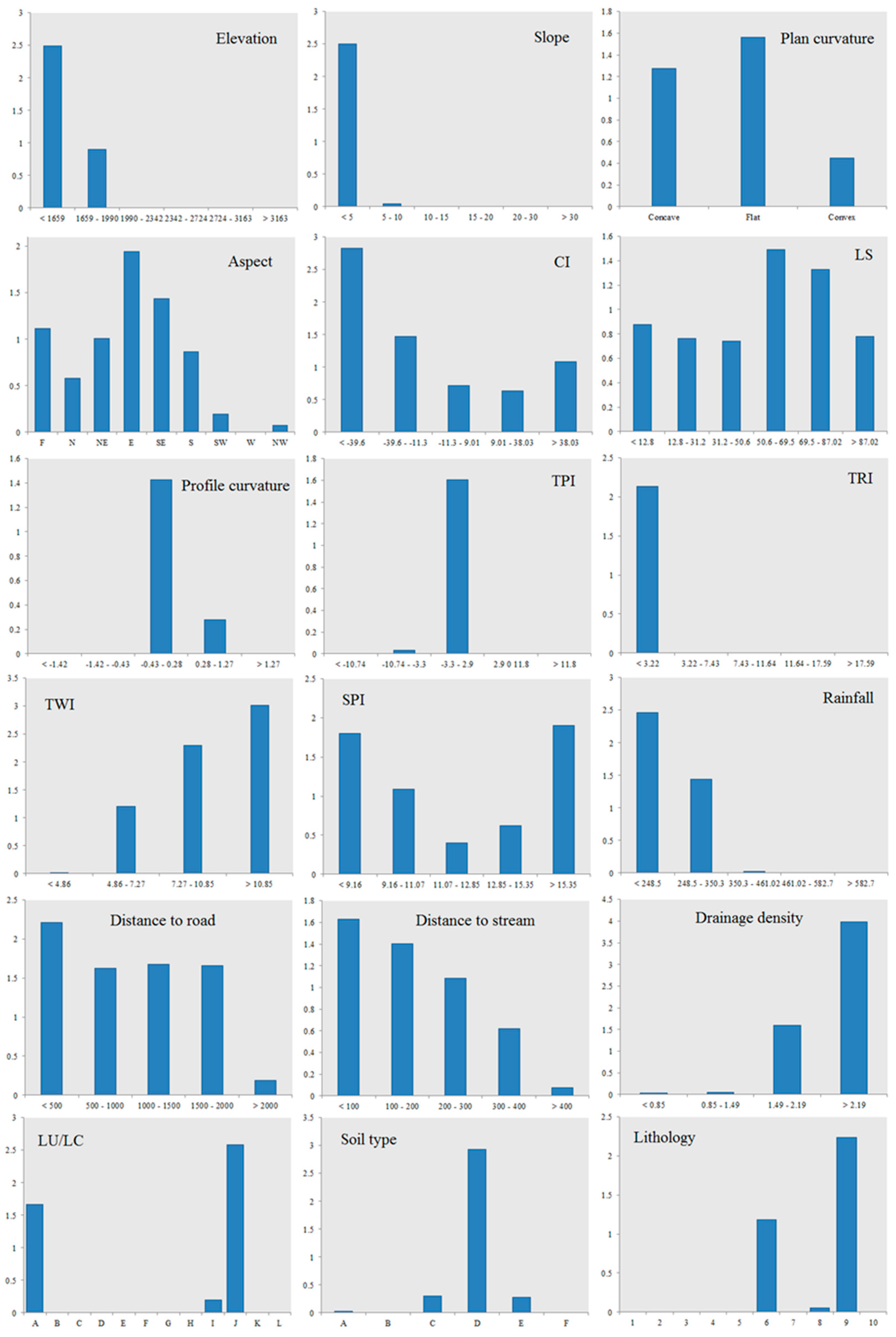
The analysis of the spatial relationship between GECFs and the gullies occurred in the study area was conducted first using the IoE and WoE models (

Table 3. The spatial relationship between gully erosion conditioning factors and gully locations.

Factor	Value	Total Pixels		Total Gullies		Weight of Evidence
		No	%	No	%	C	S©	C/S©
Elevation (m)	<1659	479814	32.482	171	81.043	2.185	0.176	12.439
	1659–1990	309671	20.964	40	18.957	−0.126	0.176	−0.716
	1990–2342	239854	16.238	0	0.000	−0.177	0.069	−2.574
	2342–2724	209109	14.156	0	0.000	−0.153	0.069	−2.218
	2724–3163	146912	9.946	0	0.000	−0.105	0.069	−1.522
	>3163	91792	6.214	0	0.000	−0.064	0.069	−0.932
Slope (°)	<5	588363	39.831	210	99.526	5.760	1.002	5.746
	5–10	149259	10.105	1	0.474	−3.162	1.002	−3.154
	10–15	124159	8.405	0	0.000	−0.088	0.069	−1.276
	15–20	143874	9.740	0	0.000	−0.102	0.069	−1.489
	20–30	280859	19.014	0	0.000	−0.211	0.069	−3.064
	>30	190637	12.906	0	0.000	−0.138	0.069	−2.007
PC	Concave	571885	38.715	104	49.289	0.431	0.138	3.129
	Flat	308591	20.891	69	32.701	0.610	0.147	4.156
	Convex	596675	40.394	38	18.009	−1.127	0.179	−6.289
Aspect	F	6262	0.424	1	0.474	0.112	1.002	0.112
	N	132304	8.957	11	5.213	−0.311	0.360	−0.862
	NE	152509	10.325	22	10.427	0.011	0.225	0.049
	E	245198	16.599	68	32.227	0.871	0.147	5.914
	SE	341071	23.090	70	33.175	0.503	0.146	3.441
	S	273880	18.541	34	16.114	−0.170	0.187	−0.906
	SW	144941	9.812	4	1.896	−1.728	0.505	−3.424
	W	89718	6.074	0	0.000	−0.063	0.069	−0.910
	NW	91269	6.179	1	0.474	−2.627	1.002	−2.621
CI	<−39.6	91462	6.223	37	17.619	1.171	0.181	6.463
	−39.6–−11.3	289807	19.717	61	29.048	0.511	0.152	3.362
	−11.3–9.01	663255	45.125	68	32.381	−0.541	0.147	−3.667
	9.01–38.03	341553	23.238	31	14.762	−0.559	0.195	−2.871
	>38.03	83751	5.698	13	6.190	0.088	0.286	0.308
LS (m)	<12.8	352071	23.834	44	20.853	−0.172	0.169	−1.015
	12.8–31.2	220640	14.937	24	11.374	−0.314	0.217	−1.446
	31.2–50.6	197564	13.375	21	9.953	−0.334	0.230	−1.454
	50.6–69.5	211467	14.316	45	21.327	0.484	0.168	2.880
	69.5–87.02	279653	18.932	53	25.118	0.362	0.159	2.282
	>87.02	215757	14.606	24	11.374	−0.287	0.217	−1.325
Profile curvature	<−1.42	39576	2.679	0	0.000	−0.027	0.069	−0.395
	−1.42–−0.43	150920	10.217	0	0.000	−0.108	0.069	−1.566
	−0.43–0.28	987589	66.858	201	95.261	2.299	0.324	7.096
	0.28–1.27	249999	16.924	10	4.739	−1.410	0.324	−4.351
	>1.27	49067	3.322	0	0.000	−0.034	0.069	−0.491
TPI	<−10.74	69120	4.679	0	0.000	−0.048	0.069	−0.696
	−10.74–−3.3	233435	15.803	1	0.474	−3.674	1.002	−3.666
	−3.3–2.9	914956	61.941	210	99.526	4.860	1.002	4.849
	2.9–11.8	201144	13.617	0	0.000	−0.146	0.069	−2.127
	>11.8	58497	3.960	0	0.000	−0.040	0.069	−0.587
TRI	<3.22	692266	46.865	211	100	0.758	0.069	11.011
	3.22–7.43	286708	19.410	0	0.000	−0.216	0.069	−3.135
	7.43–11.64	285453	19.325	0	0.000	−0.215	0.069	−3.120
	11.64–17.59	174864	11.838	0	0.000	−0.126	0.069	−1.830
	>17.59	37860	2.563	0	0.000	−0.026	0.069	−0.377
TWI	<4.86	582464	39.432	1	0.474	−4.918	1.002	−4.906
	4.86–7.27	585130	39.612	101	47.867	0.336	0.138	2.441
	7.27–10.85	237436	16.074	78	36.967	1.119	0.143	7.848
	>10.85	72122	4.883	31	14.692	1.211	0.194	6.226
SPI	<9.16	322599	21.839	83	39.336	0.842	0.141	5.975
	9.16–11.07	437271	29.602	68	32.227	0.123	0.147	0.835
	11.07–12.85	455113	30.810	26	12.322	−1.153	0.209	−5.507
	12.85–15.35	203521	13.778	18	8.531	−0.539	0.246	−2.185
	>15.35	58648	3.970	16	7.583	0.686	0.260	2.636
Rainfall (mm)	<248.5	284466	19.258	100	47.393	1.329	0.138	9.641
	248.5–350.3	535319	36.240	110	52.133	0.650	0.138	4.720
	350.3–461.02	321491	21.764	1	0.474	−4.068	1.002	−4.058
	461.02–582.7	208018	14.082	0	0.000	−0.152	0.069	−2.205
	>582.7	127857	8.656	0	0.000	−0.091	0.069	−1.315
Dis to road (m)	<500	224545	15.201	71	33.649	1.040	0.146	7.139
	500–1000	193768	13.118	45	21.327	0.585	0.168	3.483
	1000–1500	166957	11.303	40	18.957	0.608	0.176	3.459
	1500–2000	147431	9.981	35	16.588	0.584	0.185	3.157
	>2000	744451	50.398	20	9.479	−2.273	0.235	−9.670
Dis to stream (m)	<100	408797	27.675	95	45.024	0.761	0.138	5.500
	100–200	298966	20.239	60	28.436	0.449	0.153	2.939
	200–300	245504	16.620	38	18.009	0.097	0.179	0.542
	300–400	157383	10.654	14	6.635	−0.518	0.277	−1.872
	>400	366502	24.811	4	1.896	−2.838	0.505	−5.622
Drainage density (km/km2)	<0.85	398195	26.957	2	0.939	−3.662	0.710	−5.155
	0.85–1.49	497684	33.692	4	1.878	−3.279	0.505	−6.497
	1.49–2.19	368973	24.979	85	39.906	0.690	0.140	4.935
	>2.19	212300	14.372	122	57.277	2.078	0.139	15.005
LU/LC	Agriculture (A)	281159	19.034	67	31.754	0.683	0.148	4.617
	Dense-forest (B)	155	0.010	0	0.000	0.000	0.069	−0.002
	Good-range (C)	8660	0.586	0	0.000	−0.006	0.069	−0.085
	Agri-dryfarming (D)	243	0.016	0	0.000	0.000	0.069	−0.002
	Dryfarming (E)	16235	1.099	0	0.000	−0.011	0.069	−0.161
	Low-forest (F)	337471	22.846	0	0.000	−0.259	0.069	−3.768
	Woodland (G)	233619	15.816	0	0.000	−0.172	0.069	−2.501
	Mod-forest (H)	83527	5.655	0	0.000	−0.058	0.069	−0.846
	Mod-range (I)	105592	7.148	3	1.422	−1.675	0.581	−2.880
	Poor-range (J)	382114	25.868	141	66.825	1.753	0.146	11.992
	Rock (K)	23154	1.567	0	0.000	−0.016	0.069	−0.230
	Urban (L)	5220	0.353	0	0.000	−0.004	0.069	−0.051
Soil type	Rock Outcrop/Entisols (A)	486282	32.920	2	0.948	−3.938	0.710	−5.542
	Alfisols (B)	7086	0.480	0	0.000	−0.005	0.069	−0.070
	Aridisols (C)	161526	10.935	7	3.318	−1.275	0.384	−3.317
	Entisols/Inceptisols (D)	479698	32.475	201	95.261	3.733	0.324	11.522
	Inceptisols (E)	24777	1.677	1	0.474	−1.276	1.002	−1.273
	Mollisols (F)	317783	21.513	0	0.000	−0.242	0.069	−3.519
Lithology	Group 1	76475	5.177	0	0.000	−0.053	0.069	−0.772
	Group 2	131673	8.914	0	0.000	−0.093	0.069	−1.356
	Group 3	114748	7.768	0	0.000	−0.081	0.069	−1.175
	Group 4	94149	6.374	0	0.000	−0.066	0.069	−0.957
	Group 5	33722	2.283	0	0.000	−0.023	0.069	−0.336
	Group 6	117907	7.982	20	9.479	0.188	0.235	0.801
	Group 7	31564	2.137	0	0.000	−0.022	0.069	−0.314
	Group 8	134059	9.076	1	0.474	−3.043	1.002	−3.036
	Group 9	594531	40.248	190	90.047	2.598	0.230	11.297
	Group 10	148324	10.041	0	0.000	−0.106	0.069	−1.537

and Figure 5). Values less than 1 in the IoE model indicate low correlations and values larger than 1 indicate higher correlations. In general, high values of IoE indicate higher probability of gully occurrence and lower values indicate less likelihood that gullying will occur [16]. Negative values generated by the WoE model indicate negative spatial relationships and positive values reflect positive relationships. Zero indicates that the specific class of conditioning factors is not useful in the analysis [70]. Classes of the factors elevation, slope, plan curvature, aspect, and CI have strong relationships with gullying in the IoE model: classes of <1659 m = 2.495, <5° = 2.499, flat curvature = 1.565, east-facing = 1.941, and CI < −39.6 = 2.831. In the WoE model, these same classes also show strong relationships with sites of gullying: <1659 m = 12.43, <5° = 5.746, flat curvature = 4.156, east-facing = 5.914, and CI < −39.6 = 6.463. With regard to the factors in the IoE model, LS, profile curvature, TPI, TRI, and TWI have strongly predictive classes: 50.6 to 69.5 m = 1.490, −0.43 to 0.28 = 1.425, −3.3 to 2.9 = 1.607, <3.22 = 2.134, and > 10.85 = 3.009. These same factors and class are similarly strongly correlated with gullying in the WoE model: 50.6 to 69.5 m = 2.880, −0.43 to 0.28 = 7.096, −3.3 to 2.9 = 4.849, <3.22 = 11.011, and >10.85 = 6.226. In the case of the IoE model, the factors SPI, rainfall, distance to road, distance to stream, and drainage density have classes that strongly indicate locations of highest susceptibility to gully erosion: > 15.35 = 1.910, <248.5 mm = 2.461, <500 m=2.214, <100 m = 1.627, and >2.19 km/km² = 3.385. In the WoE model these same classes indicated high susceptibility as well: > 15.35 = 2.636, <248.5 mm = 9.641, < 500 m = 7.139, <100 m = 5.500, and >2.19 km/km² = 15.005). The IoE model aligns classes of LU/LC, soil type, and lithology with higher susceptibility: poor rangeland = 2.583, entisols/inceptisols = 2.933, and Group 9 (consisting of quaternary formations that include high elevation piedmont fan and valley terrace deposits, stream channel, braided channel, and floodplain deposits, low elevation piedmont fan and valley terrace deposits = 2.237. The same classes in the WoE model are highly predictive of gullying, as well: poor rangeland = 11.992, entisols/inceptisols = 11.522, and group 9 = 11.297.

3.3. Determining the Relative Importance of GECFs in the IoE Model

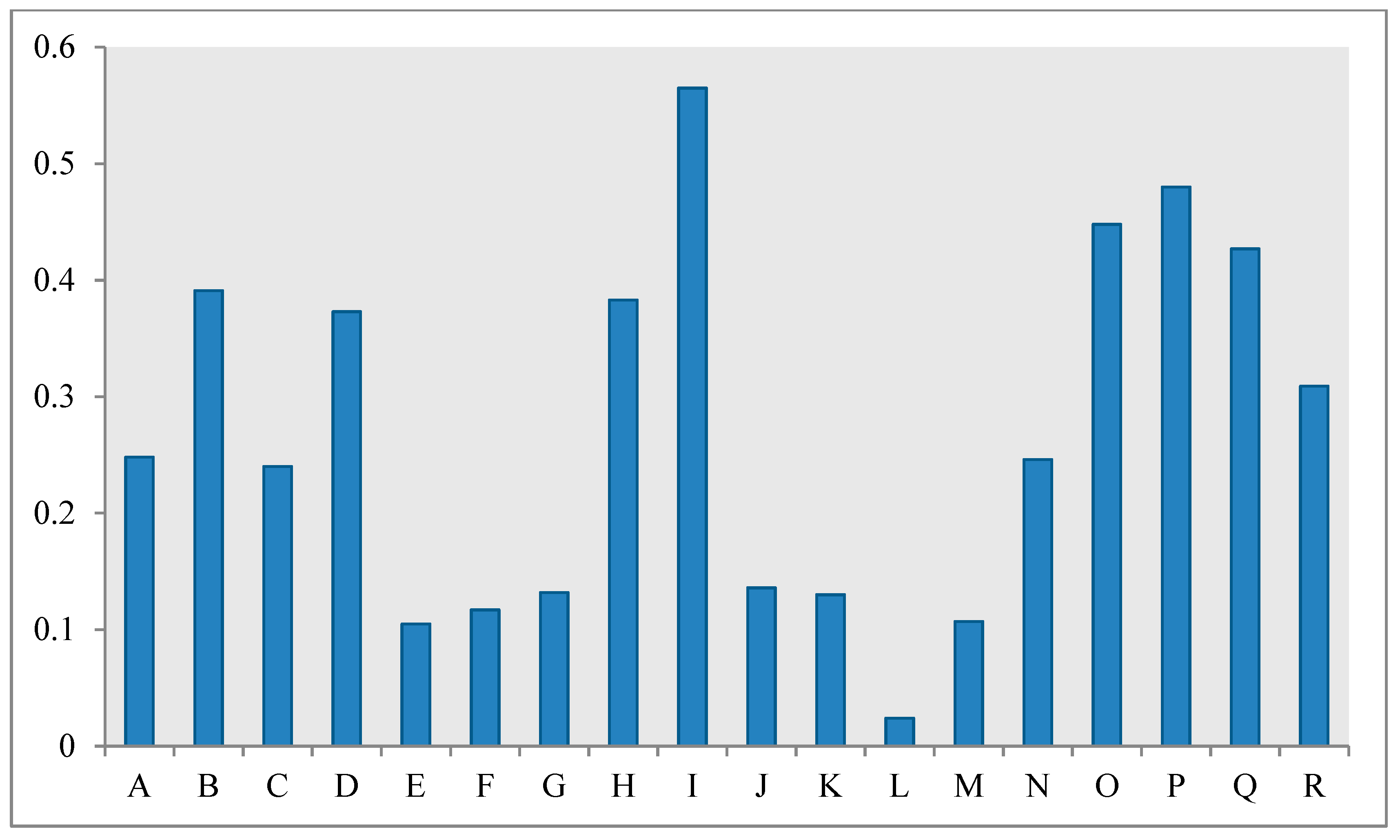
The order of importance of the GECFs in the IoE model (Figure 6) is: drainage density (0.564), slope (0.48), rainfall (0.448), TRI (0.427), soil type (0.391), elevation (0.383), TWI (0.373), TPI (0.309), LU/LC (0.248), profile curvature (0.246), lithology (0.24), distance to road (0.136), CI (0.132), distance to stream (0.13), slope aspect (0.117), plan curvature (0.107), SPI (0.105), and LS (0.024).

3.4. Gully Erosion Susceptibility Mapping (GESM)

After the computation of the spatial relationship between gully erosion and conditioning factors, and determination of the relative importance of GECFs in the IoE model, GESM calculations based on the WoE model Equation (15), the IoE model Equation (16), and the hybrid WoE- IoE model Equation (17) were constructed.

$$\begin{array}{ll}{\mathrm{GESM}}_{\mathrm{WoE}}=& \left({\mathrm{W}}_{\mathrm{WoE}}\mathrm{Elevation}\right)+\left({\mathrm{W}}_{\mathrm{WoE}}\mathrm{Slope}\right)+\left({\mathrm{W}}_{\mathrm{WoE}}\mathrm{Plan}\mathrm{curvature}\right)\\ & \hspace{1em}+\left({\mathrm{W}}_{\mathrm{WoE}}\mathrm{Slope}\mathrm{aspect}\right)+\left({\mathrm{W}}_{\mathrm{WoE}}\mathrm{CI}\right)+\left({\mathrm{W}}_{\mathrm{WoE}}\mathrm{LS}\right)\\ & \hspace{1em}+\left({\mathrm{W}}_{\mathrm{WoE}}\mathrm{Profile}\mathrm{curvature}\right)+\left({\mathrm{W}}_{\mathrm{WoE}}\mathrm{TPI}\right)+\left({\mathrm{W}}_{\mathrm{WoE}}\mathrm{TRI}\right)\\ & \hspace{1em}+\left({\mathrm{W}}_{\mathrm{WoE}}\mathrm{TWI}\right)+\left({\mathrm{W}}_{\mathrm{WoE}}\mathrm{SPI}\right)+\left({\mathrm{W}}_{\mathrm{WoE}}\mathrm{Rainfall}\right)\\ & \hspace{1em}+\left({\mathrm{W}}_{\mathrm{WoE}}\mathrm{Distance}\mathrm{to}\mathrm{road}\right)+\left({\mathrm{W}}_{\mathrm{WoE}}\mathrm{Distance}\mathrm{to}\mathrm{stream}\right)\\ & \hspace{1em}+\left({\mathrm{W}}_{\mathrm{WoE}}\mathrm{Drinage}\mathrm{density}\right)+\left({\mathrm{W}}_{\mathrm{WoE}}\mathrm{LU}/\mathrm{LC}\right)+\left({\mathrm{W}}_{\mathrm{WoE}}\mathrm{Soil}\mathrm{type}\right)\\ & \hspace{1em}+\left({\mathrm{W}}_{\mathrm{WoE}}\mathrm{Lithology}\right)\end{array}$$

(15)

$$\begin{array}{ll}{\mathrm{GESM}}_{\mathrm{IoE}}=& \left({\mathrm{W}}_{\mathrm{IoE}}\mathrm{Elevation}\times 0.383\right)+\left({\mathrm{W}}_{\mathrm{IoE}}\mathrm{Slope}\times 0.48\right)\\ & \hspace{1em}+\left({\mathrm{W}}_{\mathrm{IoE}}\mathrm{Plan}\mathrm{curvature}\times 0.107\right)+\left({\mathrm{W}}_{\mathrm{IoE}}\mathrm{Slope}\mathrm{aspect}\times 0.117\right)\\ & \hspace{1em}+\left({\mathrm{W}}_{\mathrm{IoE}}\mathrm{CI}\times 0.132\right)+\left({\mathrm{W}}_{\mathrm{IoE}}\mathrm{LS}\times 0.024\right)\\ & \hspace{1em}+\left({\mathrm{W}}_{\mathrm{IoE}}\mathrm{Profile}\mathrm{curvature}\times 0.246\right)+\left({\mathrm{W}}_{\mathrm{IoE}}\mathrm{TPI}\times 0.309\right)\\ & \hspace{1em}+\left({\mathrm{W}}_{\mathrm{IoE}}\mathrm{TRI}\times 0.427\right)+\left({\mathrm{W}}_{\mathrm{IoE}}\mathrm{TWI}\times 0.373\right)+\left({\mathrm{W}}_{\mathrm{IoE}}\mathrm{SPI}\times 0.105\right)\\ & \hspace{1em}+\left({\mathrm{W}}_{\mathrm{IoE}}\mathrm{Rainfall}\times 0.448\right)+\left({\mathrm{W}}_{\mathrm{IoE}}\mathrm{Distance}\mathrm{to}\mathrm{road}\times 0.136\right)\\ & \hspace{1em}+\left({\mathrm{W}}_{\mathrm{IoE}}\mathrm{Distance}\mathrm{to}\mathrm{stream}\times 0.13\right)+\left({\mathrm{W}}_{\mathrm{IoE}}\mathrm{Drinage}\mathrm{density}\times 0.565\right)\\ & \hspace{1em}+\left({\mathrm{W}}_{\mathrm{IoE}}\mathrm{LU}/\mathrm{LC}\times 0.248\right)+\left({\mathrm{W}}_{\mathrm{IoE}}\mathrm{Soil}\mathrm{type}\times 0.391\right)\\ & \hspace{1em}+\left({\mathrm{W}}_{\mathrm{IoE}}\mathrm{Lithology}\times 0.24\right)\end{array}$$

(16)

$$\begin{array}{ll}{\mathrm{GESM}}_{\mathrm{WoE}-\mathrm{IoE}}=& \left({\mathrm{W}}_{\mathrm{WoE}}\mathrm{Elevation}\times 0.383\right)+\left({\mathrm{W}}_{\mathrm{WoE}}\mathrm{Slope}\times 0.48\right)\\ & \hspace{1em}+\left({\mathrm{W}}_{\mathrm{WoE}}\mathrm{Plan}\mathrm{curvature}\times 0.107\right)+\left({\mathrm{W}}_{\mathrm{WoE}}\mathrm{Slope}\mathrm{aspect}\times 0.117\right)\\ & \hspace{1em}+\left({\mathrm{W}}_{\mathrm{WoE}}\mathrm{CI}\times 0.132\right)+\left({\mathrm{W}}_{\mathrm{WoE}}\mathrm{LS}\times 0.024\right)\\ & \hspace{1em}+\left({\mathrm{W}}_{\mathrm{WoE}}\mathrm{Profile}\mathrm{curvature}\times 0.246\right)+\left({\mathrm{W}}_{\mathrm{WoE}}\mathrm{TPI}\times 0.309\right)\\ & \hspace{1em}+\left({\mathrm{W}}_{\mathrm{WoE}}\mathrm{TRI}\times 0.427\right)+\left({\mathrm{W}}_{\mathrm{WoE}}\mathrm{TWI}\times 0.373\right)\\ & \hspace{1em}+\left({\mathrm{W}}_{\mathrm{WoE}}\mathrm{SPI}\times 0.105\right)+\left({\mathrm{W}}_{\mathrm{WoE}}\mathrm{Rainfall}\times 0.448\right)\\ & \hspace{1em}+\left({\mathrm{W}}_{\mathrm{WoE}}\mathrm{Distance}\mathrm{to}\mathrm{road}\times 0.136\right)+\left({\mathrm{W}}_{\mathrm{WoE}}\mathrm{Distance}\mathrm{to}\mathrm{stream}\times 0.13\right)\\ & \hspace{1em}+\left({\mathrm{W}}_{\mathrm{WoE}}\mathrm{Drinage}\mathrm{density}\times 0.565\right)+\left({\mathrm{W}}_{\mathrm{WoE}}\mathrm{LU}/\mathrm{LC}\times 0.248\right)\\ & \hspace{1em}+\left({\mathrm{W}}_{\mathrm{WoE}}\mathrm{Soil}\mathrm{type}\times 0.391\right)+\left({\mathrm{W}}_{\mathrm{WoE}}\mathrm{Lithology}\times 0.24\right).\end{array}$$

(17)

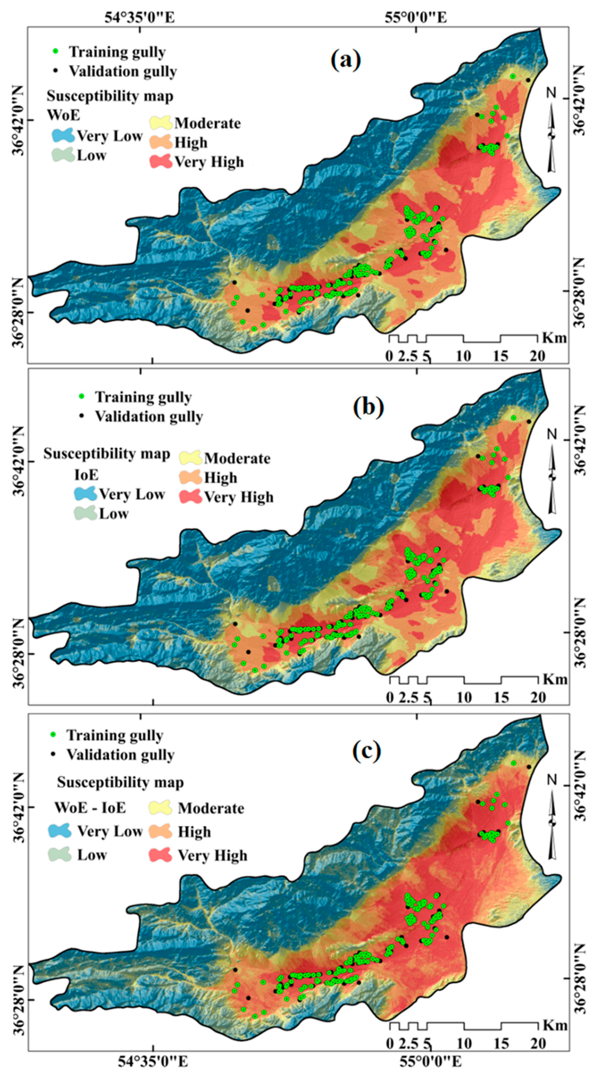
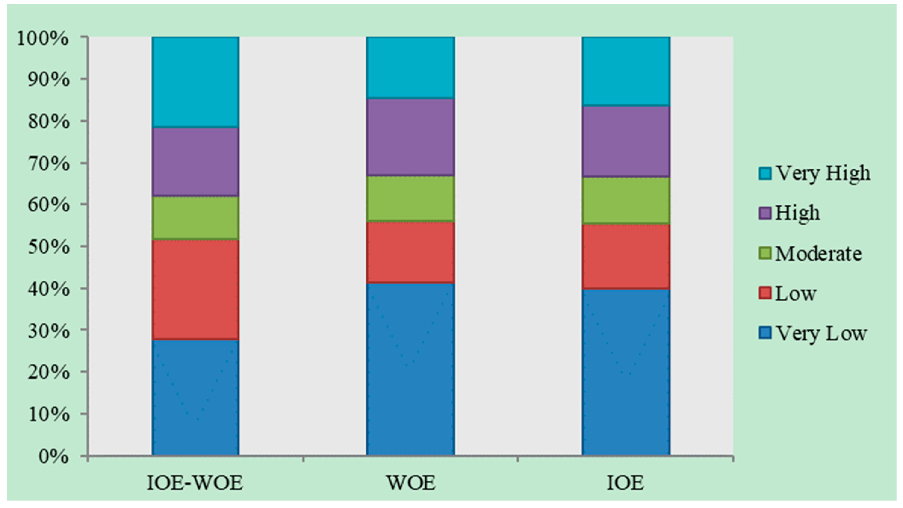
Values of gully erosion susceptibility for the WoE model, the IoE model, and the hybrid WoE-IoE model varied for the minimums (−77.558, 0.265, and −23.3362) and the maximums (143.404, 13.810, and 51.6535) of each, respectively. These values were classified into five classes using the natural breaks method: very low, low, moderate, high, and very high susceptibility classes (Figure 7a–c). The results for each category using the WoE model were 41.45%, 14.59%, 10.91%, 18.5%, and 14.52%, respectively (Figure 8). The results for each category using the IoE model were 40.03%, 15.43%, 11.10%, 17.18%, and 16.22%, respectively (Figure 8). And using WoE-IoE integrated model, the classes of susceptibility were 27.95%, 23.78%, 10.22%, 16.60%, and 21.42%, respectively.

3.5. Validation of Results

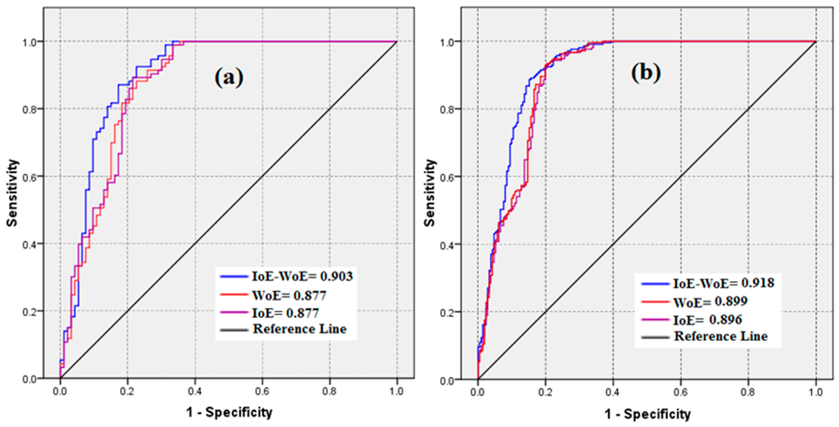
The AUROC graphs were created for the training dataset (success-rate curve) and for the validation dataset (prediction-rate curve) (Figure 9a,b). These demonstrate that the WoE model had better performance in terms of the success-rate curve (SRC = 0.899) than did the IoE model (SRC = 0.896). The results also indicate that integration of these models improve their performance: the WoE-IoE integrated model had a better prediction-rate curve (PRC = 0.903) and a better success-rate curve (SRC = 0.918) than either the WoE (PRC = 0.877 and SRC = 0.877) or IoE (PRC = 0.899 and SRC = 0.896).

4. Discussion

In terms of the position of the gully in the landscape [71], most of the gullies are on the floor of the valley and in terms of the evolution of the gullies [72], most are continuous. The continuous gully is part of the drainage network, and a discontinuous gully is separated from the drainage network. In terms of gully head-cut plan [73,74], the gullies in the study area are the digitized type, usually found adjacent to rivers and often located at the intersection of their branches. These gullies form in areas of 0% to 5% slope. The most important factors that led to the development of gullies in the study area are: the undercutting of the boundaries of flood flows and gravitational formation of mass fractures; formation of a groove in gullies due to rill erosion and the resulting surface runoff; the influences of tunnel erosion (piping) and underground corridors which have a maximum diameter of 8 meters and a maximum length of 12 m—the expansion of these corridors and the collapse of their roofs cause gully development; and head-cut retrogradation and upward development of gullies.

Determination of the susceptible areas affected by different kinds of soil erosion such as gully erosion is useful for land use planning, mitigating soil erosion, and conservation practices [29]. So far, various methods have been applied for gully erosion susceptibility assessment globally [28,29,30]. Given the shortcomings and limitations of each of the models, scientists have proposed and developed integrated methods to overcome their disadvantages and increase their efficiency [14]. In this study, two types of statistical methods, namely, IoE and WoE, and their ensemble were applied to produce GESM. The IoE–WoE integrated method eliminates the disadvantages of IoE and WoE individual models and improves their advantages. The main advantages of the WoE method are that it calculates the weighted value of the factors based on a statistical formula and thus avoids the subjective choice of weighting factors. In addition, input maps with missing data (incomplete coverage) can be accommodated in the model and under-sampled data do not significantly impact the results. The main shortcomings of the model are the failure to calculate the relative importance of the parameters, and that the weighted values calculated for different areas are not comparable in terms of the degree of hazard [31]. The main advantage of IoE model is that this model does not require that assumptions be made about the proper distribution of explanatory variables; therefore, several properties can be used and tested. This method also examines the statistical relationships between independent and dependent variables and provides metrics for the significance of variables [30].

Analyses of the spatial relationships between GECFs and gully locations using IoE, and WoE show that areas of low elevation and slope and flat topography, where surface runoff concentrates and where erosion-sensitive evaporation deposits of gypsum or salt have formed, have a high susceptibility to gully erosion. This has been demonstrated in other local studies [69,75]. Areas nearer to streams and roads, with sparse vegetation and higher drainage density than other areas, have more potential for gully occurrence. These findings are in line with References [22,76]. Limestone, sandstone, marl, shale, and red conglomerate geological units have a high susceptibility to gully erosion. These geomorphological features are generally known to promote gully erosion; this is confirmed within the study area and has been reported in other research [77,78].

The IoE model has shown that drainage density, slope degree, and rainfall are key conditional factors for gully erosion in the study area. This is in line with References [16,63,79]. Yesilnacar et al. [79] proved that gently sloping areas are susceptible to surface flow accumulation and gully erosion. Pourghasemi et al. [63] assessed the capability of WoE and FR models for spatial prediction of gully erosion susceptibility in the Chavar region of Ilam Province, Iran. Sixty-three gullies and ten GECFs were used in that study. Their results indicate that the distance to roads, drainage density, and LU/LC are key conditions affecting gully occurrence. Arabameri et al. [16] compared three data-driven models and an AHP knowledge-based technique for gully-erosion susceptibility mapping in the Toroud watershed in Semnan Province, Iran using 80 gully locations and 13 GECFs (including elevation, slope degree, slope aspect, plan curvature, distance from river, drainage density, distance from road, lithology, LU/LC, TWI, SPI, NDVI, and LS). Their results show that lithology, slope, and NDVI are the primary determinants of gully occurrence in the Toroud watershed.

Validation results show that the IoE model performed better than the WoE model. This is consistent with the work of others [16,80,81]. Arabameri et al. [16] States that IoE with an SRC = 0.939 and a PRC = 0.925 better predicts areas prone to gully erosion than does WoE with an SRC = 0.926 and a PRC = 0.921. Wang et al. [81] used IoE and FR models for groundwater qanat potential mapping in the Moghan watershed, Iran and their results depict the excellence of IoE model in qanat occurrence potential estimation. The integration of WoE and IoE has improved upon their separate performances, which is also consistent with References [14,39,82,83,84,85,86,87,88]. Arabameri et al. [14] used EBF, LR, and a new ensemble EBF–LR algorithm to spatially model gully erosion at Semnan Province, Iran. Their results show that their ensemble method performed considerably better (AUC = 0.909) than did the individual LR (0.802) and EBF (0.821) methods. Pourghasemi et al. [39] assessed the individual and ensemble data-mining techniques for gully erosion modeling and stated that the ensemble models had a higher goodness-of-fit and predictive power than individual models. Arabameri et al. [84] compared the performance of individual and ensemble models for assessment of landslide susceptibility in Sangtarashan watershed, Mazandran Province, Iran and state that FR–RF integrated model (AUC = 0.917) achieved higher predictive accuracy than the individual FR (AUC = 0.865) and RF (AUC = 0.840) models. Du et al. [85] integrated IV and LR individual models for landslide susceptibility mapping in the Bailongjiang watershed, Gansu Province, China and state that the proposed integrated method was reliable to produce an accurate landslide susceptibility map. [88] Used ensemble RF and EBF models for landslide susceptibility assessment in Western Mazandaran Province, Iran and state that introduced ensemble model can be a powerful tool for landslide assessment at regional scales.

Our research will contribute to achieve a better knowledge of the landscape and to develop sustainable policies to achieve the Land Degradation Neutrality challenge and the United Nation Goals for Land Degradation [89,90]. This is a relevant issue to achieve sustainable land management where gullies must be restored when developed as a consequence of human mismanagement, and for this is necessary to use nature-based solutions [91]. To achieve success in gully erosion control the strategies must find a way to reduce the connectivity of the flows [92].

5. Conclusions

Gully erosion is a common geomorphological problem in arid and semi-arid regions, therefore, it is essential to develop methods for predicting gullying with highly accurate and effective models. Knowing the locations that are prone to or susceptible to gullying can enable ways to avoid casualties and financial losses caused by gully development, and can even promote sustainable development. In recent years, many quantitative and qualitative methods have been introduced for GESM. No approach is believed to be a best-approach, but the general consensus is that each method has its advantages and disadvantages. In this study, two models (the IoE and the WoE) and their integrated offspring (WoE-IoE) were tested for GESM to assess what their advantages and shortcomings were. The most important conclusions to be drawn from this study are:

• Based on extensive field surveys and multicollinearity tests, topographical, hydrological, geological, soil characteristics, and environmental factors are significant factors that influence gullying in the study area.
• Spatial comparisons of GECFs and gullies using IoE and WoE models show that areas with low elevations, low slopes, and flat topography concentrate surface runoff, and areas near streams and roads, having sparse vegetation, and higher drainage densities have greater potential for gully occurrence.
• By using the IoE model to determine the relative importance of GECFs, we have revealed that drainage density, slope degree, and rainfall are key conditional factors for gully erosion in the study area.
• Validation showed that integration of the WoE and IoE models improves the performance of either of them individually, but also decreases the disadvantages inherent in each. The WoE-IoE integrated model had higher prediction accuracy than the WoE and IoE models.
• Integration of the WoE and IoE models and use of remote sensing data and GIS technique be a powerful tool for GESM and have excellent accuracy.
• The novel method introduced in this research is adaptable and can be used in other areas.
• Our approach can be used to control the growth of the gullies when human-induced.

References

- Peugeot, S.; Cappelare, B.; Vieux, B.E.; Seguis, L.; Maia, A. Hydrologic process simulation of a semiarid endoreic catchment in Sahelan west, model-aided data analysis and screening. J. Hydrol. 2003, 279, 224–243. [Google Scholar] [CrossRef]
- Boardman, J.; Parsons, A.J.; Holland, R.; Holmes, P.J. Development of Badlands and Gullies in the Sneeuberg; Catena: Great Karoo, South Africa, 2003; Volume 50, pp. 165–184. [Google Scholar]
- McIntosh, P.; Mike, L. Soil erodibility and erosion hazard: Extending these cornerstone soil conservation oncepts to headwater streams in the forestry estate in Tasmania. For. Ecol. Manag. 2005, 220, 128–139. [Google Scholar] [CrossRef]
- Amsler, L.M.; Ramonell, C.G.; Toniolo, H.A. Morphologic changes in the Parana river channel in the li ght of the climate variability during the 20the century. Geomorphology 2005, 65, 56–70. [Google Scholar]
- Marker, M.; Angeli, L.; Bottai, L.; Costantini, R. Assessment of land degradation susceptibility by scenario analysis. Geomorphology 2008, 93, 120–129. [Google Scholar] [CrossRef]
- Zhou, P. Effect of vegetation cover on soil erosion in a mountainous watershed. Catena 2008, 75, 319–325. [Google Scholar] [CrossRef]
- Battagli, S.A.; Leoni, L.; Sartori, F. Mineralogical and grain size composition of clays developing calanchi and biancane erosional landforms. Geomorphology 2002, 49, 153–170. [Google Scholar] [CrossRef]
- Borrelli, P.; Märker, M.; Panagos, P.; Schütt, B. Modeling soil erosion and river sediment yield for an intermountain drainage basin of the Central Apennines, Italy. Catena 2014, 114, 45–58. [Google Scholar]
- Luffman, I.E.; Nandi, A.; Spiegel, T. Gully morphology, hillslope erosion, and precipitation characteristics in the Appalachian Valley and Ridge province, southeastern USA. Catena 2015, 133, 221–232. [Google Scholar] [CrossRef]
- Rafaello, B.; Reis, E. Controlling factors of the size and location of large gully systems: A regression based exploration using reconstructed pre-erosion topography. Catena 2016, 147, 621–631. [Google Scholar]
- Poesen, J.; Nachtergaele, J.; Verstraeten, G.; Valentin, C. Gully Erosion and Environment Change: Importance and Research Needs. Catena 2003, 50, 91–133. [Google Scholar] [CrossRef]
- Frankl, A.; Deckers, J.; Moulaert, L.; Van Damme, A.; Haile, M.; Poesen, J.; Nyssen, J. Integrated solutions for combating gully erosion in areas prone to soil piping: Innovations from the drylands of Northern Ethiopia. Land Degrad. Dev. 2014, 27, 1797–1804. [Google Scholar] [CrossRef]
- Meliho, M.; Khattabi, A.; Mhammdi, N. A GIS-based approach for gully erosion susceptibility modeling using bivariate statistics methods in the Ourika watershed, Morocco. Environ. Earth Sci. 2018, 77, 655. [Google Scholar] [CrossRef]
- Arabameri, A.; Pradhan, B.; Rezaei, K.; Yamani, M.; Pourghasemi, H.R.; Lombardo, L. Spatial modeling of gully erosion using Evidential Belief Function, Logistic Regression and a new ensemble EBF–LR algorithm. Land Degrad. Dev. 2018, 29, 4035–4049. [Google Scholar] [CrossRef]
- Arabameri, A.; Pradhan, B.; Pourghasemi, H.R.; Rezaei, K.; Kerle, N. Spatial Modeling of Gully Erosion Using GIS and R Programing: A Comparison among Three Data Mining Algorithms. Appl. Sci. 2018, 8, 1369. [Google Scholar] [CrossRef]
- Arabameri, A.; Rezaei, K.; Pourghasemi, H.R.; Lee, S.; Yamani, M. GIS-based gully erosion susceptibility mapping: A comparison among three data-driven models and AHP knowledge-based technique. Environ. Earth Sci. 2018, 77, 628. [Google Scholar] [CrossRef]
- Arabameri, A.; Pourghasemi, H.R. Spatial Modeling of Gully Erosion Using Linear and Quadratic Discriminant Analyses in GIS and R. In Spatial Modeling in GIS and R for Earth and Environmental Sciences, 1st ed.; Pourghasemi, H.R., Gokceoglu, C., Eds.; Elsevier Publication: Amsterdam, The Netherlands, 2019; p. 796. [Google Scholar]
- Nwankwo, C.; Nwankwoala, H.O. Gully Erosion Susceptibility Mapping in Ikwuano Local Government Area of Abia State, Nigeria Using GIS Techniques. Earth Sci. Malaysis 2018, 2, 08–15. [Google Scholar]
- Azareh, A.; Rahmati, O.; Rafiei-Sardooi, E.; Sankey, J.B.; Lee, S.; Shahabi, H.; BinAhmad, B. Modeling gully-erosion susceptibility in a semi-arid region, Iran: Investigation of applicability of certainty factor and maximum entropy models. Sci. Total Environ. 2019, 655, 684–696. [Google Scholar] [CrossRef] [PubMed]
- Nachtergaele, J.; Poesen, J.; Sidorchuk, A.; Torri, D. Prediction of concentrated flow width in ephemeral gully channels. Hydrol. Process. 2002, 16, 1935–1953. [Google Scholar] [CrossRef]
- Saynor, M.J.; Erskine, W.D.; Evans, K.G.; Eliot, I. Gully ignition and implication for management of scour holes in the vicinity of the jabiluka mine, Australia. Geogr. Ann. 2004, 86, 19–201. [Google Scholar] [CrossRef]
- Campo-Bescós, M.; Flores-Cervantes, J.; Bras, R.; Casalí, J.; Giráldez, J. Evaluation of a gully headcut retreat model using multitemporal aerial photographs and digital elevation models. J. Geophys. Res. Earth Surf. 2013, 118, 2159–2173. [Google Scholar] [CrossRef] [Green Version]
- Conoscenti, C.; Angileri, S.; Cappadonia, C.; Rotigliano, E.; Agnesi, V.; Märker, M. Gully erosion susceptibility assessment by means of GIS-based logistic regression: A case of Sicily (Italy). Geomorphology 2014, 204, 399–411. [Google Scholar] [CrossRef] [Green Version]
- Chaplot, V.; Giborie, G.; Marchand, P.; Valentin, C. Dynamic modeling for linear erosion intiation and development under climate and land-use changes in northen Laos. Catena 2005, 63, 318–328. [Google Scholar] [CrossRef]
- Dotter weich, M. High resolution reconstruction of a 1300 year old gully system in northern Bararian. Holocene 2005, 15, 997–1005. [Google Scholar]
- Rescher, N. The Stochastic revolution and the nature of scientific explanation. Synthese 1962, 14, 200–215. [Google Scholar] [CrossRef]
- Derose, R.C.; Gomez, B.; Marden, M.; Trustrum, N.A. Gully erosion in Mangatu Forest, New Zealand, estimated from digital elevation models. Earth Surf. Process. Landf. 1998, 23, 1045–1053. [Google Scholar] [CrossRef]
- Rahmati, O.; Tahmasebipour, N.; Haghizadeh, A.; Pourghasemi, H.R.; Feizizadeh, B. Evaluating the influence of geo-environmental factors on gully erosion in a semi-arid region of Iran: An integrated framework. Sci. Total Environ. 2017, 579, 913–927. [Google Scholar] [CrossRef]
- Arabameri, A.; Pradhan, B.; Rezaei, K. Spatial prediction of gully erosion using ALOS PALSAR data and ensemble bivariate and data mining models. Geosci. J. 2019, 1–18. [Google Scholar] [CrossRef]
- Zabihi, M.; Mirchooli, F.; Motevalli, A.; Darvishan, A.K.; Pourghasemi, H.R.; Zakeri, M.A.; Sadighi, F. Spatial modeling of gully erosion in Mazandaran Province, northern Iran. Catena 2018, 161, 1–13. [Google Scholar] [CrossRef]
- Dube, F.; Nhapi, I.; Murwira, A.; Gumindoga, W.; Goldin, J.; Mashauri, D.A. Potential of weight of evidence modeling for gully erosion hazard assessment in Mbire District—Zimbabwe. Phys. Chem. Earth 2014, 67, 145–152. [Google Scholar] [CrossRef]
- Hosseinalizadeh, M.; Kariminejad, N.; Chen, W.; Pourghasemi, H.R.; Alinejad, M.; Behbahani, A.M.; Tiefenbacher, J.P. Gully headcut susceptibility modeling using functional trees, naïve Bayes tree, and random forest models. Geoderma 2019, 342, 1–11. [Google Scholar] [CrossRef]
- Kornejady, A.; Heidari, K.; Nakhavali, M. Assessment of landslide susceptibility, semi-quantitative risk and management in the Ilam dam basin, Ilam. Iran. Environ. Resour. Res. 2015, 3, 85–109. [Google Scholar]
- Rahmati, O.; Tahmasebipour, N.; Haghizadeh, A.; Pourghasemi, H.R.; Feizizadeh, B. Evaluation of different machine learning models for predicting and mapping the susceptibility of gully erosion. Geomorphology 2017, 298, 118–137. [Google Scholar] [CrossRef]
- Amiri, M.; Pourghasemi, H.R.; Ghanbarian, G.A.; Afzali, S.F. Assessment of the importance of gully erosion effective factors using Boruta algorithm and its spatial modeling and mapping using three machine learning algorithms. Geoderma 2019, 340, 55–69. [Google Scholar] [CrossRef]
- Hosseinalizadeh, M.; Kariminejad, N.; Chen, W.; Pourghasemi, H.R.; Alinejad, M.; Behbahani, A.M.; Tiefenbacher, J.P. Spatial modeling of gully headcuts using UAV data and four best-first decision classifier ensembles (BFTree, Bag-BFTree, RS-BFTree, and RF-BFTree). Geomorphology 2019, 329, 184–193. [Google Scholar] [CrossRef]
- Arabameri, A.; Pradhan, B.; Rezaei, K. Gully erosion zonation mapping using integrated geographically weighted regression with certainty factor and random forest models in GIS. J. Environ. Manag. 2019, 232, 928–942. [Google Scholar] [CrossRef]
- Hosseinalizadeh, M.; Kariminejad, N.; Rahmati, O.; Keesstra, S.; Alinejad, M.; Behbahani, A.M. How can statistical and artificial intelligence approaches predict piping erosion susceptibiIIlity? Sci. Total Environ. 2019, 646, 1554–1566. [Google Scholar] [CrossRef] [PubMed]
- Pourghasemi, H.R.; Yousefi, S.; Kornejady, A.; Cerdà, A. Performance assessment of individual and ensemble data-mining techniques for gully erosion modeling. Sci. Total Environ. 2017, 609, 764–775. [Google Scholar] [CrossRef] [Green Version]
- Shirani, K.; Pasandi, M.; Arabameri, A. Landslide susceptibility assessment by Dempster–Shafer and Index of Entropy models, Sarkhoun basin, Southwestern Iran. Nat. Hazards 2018, 93, 1379–1418. [Google Scholar] [CrossRef]
- Xie, Z.; Chen, G.; Meng, X.; Zhang, Y.; Qiao, L.; Tan, L. A comparative study of landslide susceptibility mapping using weight of evidence, logistic regression and support vector machine and evaluated by sbas-insar monitoring: Zhouqu to wudu segment in Bailong River Basin, China. Environ. Earth Sci. 2017, 76, 313. [Google Scholar] [CrossRef]
- Tien Bui, D.; Shahabi, H.; Shirzadi, A.; Chapi, K.; Alizadeh, M.; Chen, W.; Mohammadi, A.; Ahmad, B.; Panahi, M.; Hong, H. Landslide detection and susceptibility mapping by airsar data using support vector machine and index of entropy models in Cameron highlands, Malaysia. Remote Sens. 2018, 10, 1527. [Google Scholar] [CrossRef]
- Haghizadeh, A.; Siahkamari, S.; Haghiabi, A.H.; Rahmati, O. Forecasting flood-prone areas using Shannon’s entropy model. J. Earth Syst. Sci. 2017, 126, 39. [Google Scholar] [CrossRef]
- Al-Abadi, A.M.; Pourghasemi, H.R.; Shahid, S.; Ghalib, H.B. Spatial Mapping of Groundwater Potential Using Entropy Weighted Linear Aggregate Novel Approach and GIS. Arabian J. Sci. Eng. 2017, 42, 1185–1199. [Google Scholar] [CrossRef]
- Arabameri, A.; Rezaei, K.; Cerda, A.; Lombardo, L.; Rodrigo-Comino, J. GIS-based groundwater potential mapping in Shahroud plain, Iran. A comparison among statistical (bivariate and multivariate), data mining and MCDM approaches. Sci. Total Environ. 2019, 658, 160–177. [Google Scholar] [CrossRef]
- I.R. of Iran Meteorological Organization (IRIMO). 2012. Available online: http://www.mazan daranmet.ir (accessed on 12 August 2018).
- Geology Survey of Iran (GSI). 1997. Available online: http://www.gsi.ir/Main/Lang_en/index.html (accessed on 12 August 2018).
- IUSS Working Group WRB. World Reference Base for Soil Resources 2014; World Soil Resources Report; FAO: Rome, Italy, 2014. [Google Scholar]
- Cama, M.; Conoscenti, C.; Lombardo, L.; Rotigliano, E. Exploring relationships between grid cell size and accuracy for debris-flow susceptibility models: A test in the Giampilieri catchment (Sicily, Italy). Environ. Earth Sci. 2016, 75, 1–21. [Google Scholar] [CrossRef]
- Parras-Alcántara, L.; Lozano-García, B.; Keesstra, S.; Cerdà, A.; Brevik, E.C. Long-term effects of soil management on ecosystem services and soil loss estimation in olive grove top soils. Sci. Total Environ. 2016, 571, 498–506. [Google Scholar] [CrossRef]
- Arabameri, A.; Pradhan, B.; Rezaei, K.; Conoscenti, C. Gully erosion susceptibility mapping using GIS-based multi-criteria decision analysis techniques. Catena 2019, 180, 282–297. [Google Scholar] [CrossRef]
- Boreggio, M.; Bernard, M.; Gregoretti, C. Evaluating the influence of gridding techniques for Digital Elevation Models generation on the debris flow routing modeling: A case study from Rovina di Cancia basin (North-eastern Italian Alps). Front. Earth Sci. 2018, 6, 89. [Google Scholar] [CrossRef]
- Wu, C.Y.; Mossa, J.; Mao, L.; Almulla, M. Comparison of different spatial interpolation methods for historical hydrographic data of the lowermost Mississipi River. Ann. GIS 2019, in press. [Google Scholar] [CrossRef]
- Gesch, D.; Oimoen, M.; Zhang, Z.; Meyer, D.; Danielson, J. Validation of the ASTER global digital elevation model version 2 over the conterminous United States. Int. Arch. Photogramm. Remote Sens. Spat. Inf. Sci. 2012, B4, 281–286. [Google Scholar] [CrossRef]
- Zhou, C.; Ge, L.E.D.; Chang, H.C. A case study of using external DEM in InSAR DEM generation. Geo-Spat. Inf. Sci. 2005, 8, 14–18. [Google Scholar] [Green Version]
- Zhang, W.; Wang, W.; Chen, L. Constructing DEM based on InSAR and the relationship between InSAR DEM’s precision and terrain factors. Energy Procedia 2012, 16, 184–189. [Google Scholar] [CrossRef]
- Arabameri, A.; Pourghasemi, H.R.; Yamani, M. Applying different scenarios for landslide spatial modeling using computational intelligence methods. Environ. Earth Sci. 2017, 76, 832. [Google Scholar] [CrossRef]
- Arabameri, A.; Pourghasemi, H.R.; Cerda, A. Erodibility prioritization of sub-watersheds using morphometric parameters analysis and its mapping: A comparison among TOPSIS, VIKOR, SAW, and CF multi-criteria decision making models. Sci. Total Environ. 2017, 613–614, 1385–1400. [Google Scholar]
- Arabameri, A.; Pradhan, B.; Pourghasemi, H.R.; Rezaei, K. Identification of erosion-prone areas using different multi-criteria decision-making techniques and GIS. Geomat. Nat. Hazards Risk 2018, 9, 1129–1155. [Google Scholar] [CrossRef] [Green Version]
- Arabameri, A.; Rezaei, K.; Cerda, A.; Conoscenti, C.; Kalantari, Z. A comparison of statistical methods and multi-criteria decision making to map flood hazard susceptibility in Northern Iran. Sci. Total Environ. 2019, 660, 443–458. [Google Scholar] [CrossRef]
- Arabameri, A.; Pradhan, B.; Rezaei, K.; Sohrabi, M.; Kalantari, Z. GIS-based landslide susceptibility mapping using numerical risk factor bivariate model and its ensemble with linear multivariate regression and boosted regression tree algorithms. J. Mt. Sci. 2019, 16, 595–618. [Google Scholar] [CrossRef]
- Arabameri, A.; Pradhan, B.; Rezaei, K.; Saro, L.; Sohrabi, M. An Ensemble Model for Landslide Susceptibility Mapping in a Forested Area. Geocarto Int. 2019. [Google Scholar] [CrossRef]
- Pourghasemi, H.R.; Mohammady, M.; Pradhan, B. Landslide susceptibility mapping using index of entropy and conditional probability models in GIS: Safarood Basin, Iran. Catena 2012, 97, 71–84. [Google Scholar] [CrossRef]
- Rahmati, O.; Haghizadeh, A.; Pourghasemi, H.R.; Noormohamadi, F. Gully erosion susceptibility mapping: The role of GISbased bivariate statistical models and their comparison. Nat. Hazards 2016, 82, 1231–1258. [Google Scholar] [CrossRef]
- Conforti, M.; Aucelli, P.P.; Robustelli, G.; Scarciglia, F. Geomorphology and GIS analysis formapping gully erosion susceptibility in the Turbolo streamcatchment (Northern Calabria, Italy). Nat. Hazards 2011, 56, 881–898. [Google Scholar] [CrossRef]
- Conoscenti, C.; Agnesi, V.; Cama, M.; Alamaru Caraballo-Arias, N.; Rotigliano, E. Assessment of Gully Erosion Susceptibility Using Multivariate Adaptive Regression Splines and Accounting for Terrain Connectivity. Land Degrad. Dev. 2018, 29, 724–736. [Google Scholar] [CrossRef]
- Romer, C.; Ferentinou, M. Shallow landslide susceptibility assessment in a semiarid environment A Quaternary catchment of KwaZulu-Natal, South Africa. Eng. Geol. 2016, 201, 29–44. [Google Scholar] [CrossRef]
- Hong, H.; Tsangaratos, P.; Ilia, I. Application of fuzzy weight of evidence and data mining techniques in construction of flood susceptibility map of Poyang County, China. Sci. Total Environ. 2018, 625, 575–588. [Google Scholar] [CrossRef] [PubMed]
- Yesilnacar, E.K. The Application of Computational Intelligence to Landslide Susceptibility Mapping in Turkey. Ph.D. Thesis, Department of Geomatics the University of Melbourne, Melbourne, Australia, 2005. [Google Scholar]
- Regmi, N.R.; Giardino, J.R.; Vitek, J.D. Modeling susceptibility to landslides using the weight of evidence approach: Western Colorado, USA. Geomorphology 2010, 115, 172–187. [Google Scholar] [CrossRef]
- Brice, J.B. Erosion and Deposition in Loess-Mantled Great Plains, Medecine Creek Drainage Basin, Nebraska. Geol. Surv. Prof. Pap. 1966, 235–339. [Google Scholar]
- Heed, B.H. Morphology of gullies in the colorado rocky mountains. Bulletin of the International Association of Scientific Hydrology. Hydrol. Sci. J. 1970, 2, 79–89. [Google Scholar]
- Ireland, H.A.; Sharpe, C.F.; Eargle, D.H. Principles of Gully Erosion in the Piedmont of South Carolina; Tech. Bull. 633.; USDA: Washington, DC, USA, 1939.
- Hongchun, Z.H.U.; Guoan, T.; Kejian, Q.; Haiying, L. Extraction and analysis of gully head of loess plateau in china based on digital elevation model. Chin. Geogr. Sci. 2014, 24, 328–338. [Google Scholar]
- Le Roux, J.J.; Sumner, P.D. Factors controlling gully development: Comparing continuous and discontinuous gullies. Land Degrad. Dev. 2012, 23, 440–449. [Google Scholar] [CrossRef]
- Nyssen, J.; Poesen, J.; Moeyersons, J.; Luyten, E.; Veyret-Picot, M.; Deckers, J.; Haile, M.; Govers, G. Impact of road building on gully erosion risk: A case study from the northern Ethiopian highlands. Earth Surf. Process. Landf. 2002, 27, 1267–1283. [Google Scholar] [CrossRef]
- Gessesse, B.; Bewket, W.; Bräuning, A. Model-based characterization and monitoring of runoff and soil erosion in response to land use/land cover changes in the Modjo watershed, Ethiopia. Land Degrad. Dev. 2015, 26, 711–724. [Google Scholar] [CrossRef]
- Gellis, A.C.; Cheama, A.; Laahty, V.; Lalio, S. Assessment of gully control structure in the rio Nutria Watershed, New Mexico. J. Am. Water Res. Assoc. 1995, 31, 633–646. [Google Scholar] [CrossRef]
- Golestani, G.; Issazadeh, L.; Serajamani, R. Lithology effects on gully erosion in Ghoori chay Watershed using RS & GIS. Int. J. Biosci. 2014, 4, 71–76. [Google Scholar]
- Wang, Q.; Li, W.; Chen, W.; Bai, H. GIS-based assessment of landslide susceptibility using certainty factor and index of entropy models for the Qianyang County of Baoji city, China. J. Earth Syst. Sci. 2015, 124, 1399–1415. [Google Scholar] [CrossRef]
- Naghibi, S.A.; Pourghasemi, H.R.; Pourtaghie, Z.S.; Rezaei, A. Groundwater qanat potential mapping using frequency ratio and Shannon’s entropy models in the Moghan Watershed, Iran. Earth Sci. Inf. 2015, 8, 171–186. [Google Scholar] [CrossRef]
- Umar, Z.; Pradhan, B.; Ahmad, A.; Neamah Jebur, M.; Shafapour Tehrani, M. Earthquake induced landslide susceptibility mapping using an integrated ensemble frequency ratio and logistic regression models in West Sumatera Province, Indonesia. Catena 2014, 118, 124–135. [Google Scholar] [CrossRef]
- ThaiPham, B.; Prakash, I.; Tien Bui, D. Spatial prediction of landslides using a hybrid machine learning approach based on Random Subspace and Classification and Regression Trees. Geomorphology 2018, 303, 256–270. [Google Scholar]
- Arabameri, A.; Pradhan, B.; Rezaei, K.; Lee, C.-W. Assessment of Landslide Susceptibility Using Statistical-and Artificial Intelligence-Based FR–RF Integrated Model and Multiresolution DEMs. Remote Sens. 2019, 11, 999. [Google Scholar] [CrossRef]
- Du, G.; Zhang, Y.; Iqbal, J. Landslide susceptibility mapping using an integrated model of information value method and logistic regression in the Bailongjiang watershed, Gansu Province, China. J. Mount. Sci. 2017, 14, 249. [Google Scholar] [CrossRef]
- Tien Bui, D.; Tuan, T.A.; Hoang, N.D.; Thanh, N.Q.; Nguyen, D.B.; Van Liem, N.; Pradhan, B. Spatial prediction of rainfall-induced landslides for the Lao Cai area (Vietnam) using a hybrid intelligssent approach of least squares support vector machines inference model and artificial bee colony optimization. Landslides 2017, 14, 447–458. [Google Scholar] [CrossRef]
- Dehnavi, A.; Aghdam, I.N.; Pradhan, B.; Morshed, V.M.H. A new hybrid model using step-wise weight assessment ratio analysis (SWARA) technique and adaptive neuro-fuzzy inference system (ANFIS) for regional landslide hazard assessment in Iran. Catena 2015, 135, 122–148. [Google Scholar] [CrossRef]
- Pourghasemi, H.R.; Kerle, N. Random forests and evidential belief function-based landslide susceptibility assessment in Western Mazandaran Province, Iran. Environ. Earth Sci. 2016, 75, 1–17. [Google Scholar] [CrossRef]
- Keesstra, S.; Mol, G.; de Leeuw, J.; Okx, J.; de Cleen, M.; Visser, S. Soil-related sustainable development goals: Four concepts to make land degradation neutrality and restoration work. Land 2018, 7, 133. [Google Scholar] [CrossRef]
- Keesstra, S.D.; Bouma, J.; Wallinga, J.; Tittonell, P.; Smith, P.; Cerdà, A.; Montanarella, L.; Quinton, J.N.; Pachepsky, Y.; van der Putten, W.H.; et al. The significance of soils and soil science towards realization of the United Nations Sustainable Development Goals. Soil 2016, 2, 111–128. [Google Scholar] [CrossRef] [Green Version]
- Keesstra, S.; Nunes, J.; Novara, A.; Finger, D.; Avelar, D.; Kalantari, Z.; Cerdà, A. The superior effect of nature based solutions in land management for enhancing ecosystem services. Sci. Total Environ. 2018, 610, 997–1009. [Google Scholar] [CrossRef] [PubMed]
- Keesstra, S.; Nunes, J.P.; Saco, P.; Parsons, T.; Poeppl, R.; Masselink, R.; Cerdà, A. The way forward: Can connectivity be useful to design better measuring and modeling schemes for water and sediment dynamics? Sci. Total Environ. 2018, 644, 1557–1572. [Google Scholar] [CrossRef]
Figure 1.
Location of the study area in Iran and Semnan province and locations of gullies used for training (black dots) and validation (green dots).
Figure 2.
Flowchart of research in the present study for gully erosion susceptibility mapping.
Figure 3.
Sample of mapped gullies in the study area.
Figure 4.
Gully erosion conditioning factors. (a) elevation, (b) slope, (c) plan curvature, (d) slope aspect, (e) convergence index (CI), (f) slope length (LS), (g) profile curvature, (h) topography position index (TPI), (i) terrain ruggedness index (TRI), (j) topography wetness index (TWI), (k) stream power index (SPI), (l) rainfall, (m) distance to road, (n) distance to stream, (o) drainage density, (p) land use/land cover, (q) soil type, and (r) lithology.
Figure 5.
The spatial relationship between conditioning factors and gully locations.
Figure 6.
The relative importance of conditioning factors in the IoE model. A: landuse/land cover, B: Soil type, C: lithology, D: topography wetness index (TWI), E: stream power index (SPI), F: aspect, G: convergence index (CI), H: elevation, I: drainage density, J: distance to stream, K: distance to stream, L: slope length (LS), M: plan curvature, N: profile curvature, O: rainfall, P: slope, Q: terrain ruggedness index (TRI), R) topography position index (TPI).
Figure 7.
Gully erosion susceptibility map. (a) weight-of-evidence (WoE) model, (b) index-of-entropy (IoE) model, and (c) WoE-IoE integrated model.
Figure 8.
Percentage of each susceptibility classes in three models of the weight of evidence, index of entropy, and WoE-IoE.
Figure 9.
Area under curve values for weight-of-evidence (WoE), index-of-entropy (IoE), and WoE-IoE models: (a) validation dataset (prediction rate curve), (b) training dataset (success rate curve).