Application of the Simple Biosphere Model 2 (SiB2) with Irrigation Module to a Typical Low-Hilly Red Soil Farmland and the Sensitivity Analysis of Modeled Energy Fluxes in Southern China

Abstract

Land surface processes are an important part of the Earth’s mass and energy cycles. The application of a land surface process model for farmland in the low-hilly red soil region of southern China continues to draw research attention. Conventional model does not perform well in the simulation of irrigated farmland, because the influence of land surface water is not considered. In this study, an off-line version of the Simple Biosphere model 2 (SiB2) was locally parameterized in a typical farmland of the low-hilly red soil region using field observations and remote sensing data. The performance of SiB2 was then evaluated through comparison to Bowen-ratio direct measurements in a second growing period of rice in 2015 (late rice from 23 July to 31 October). The results show that SiB2 underestimated latent heat flux (LE) by 16.0% and overestimated sensible heat flux (H) by 16.7%, but net radiation flux (Rn) and soil heat flux were reasonably simulated. The single factor sensitivity analysis of Rn, H, and LE modeled in SiB2 indicated that downward shortwave radiation (DSR) and downward longwave radiation (DLR) had a significant effect on Rn simulation. In driving data, DSR, DLR and wind speed (u) were the main factors that could cause a distinct change in sensible heat flux. An irrigation module was added to the original SiB2 model to simulate the influence of irrigated paddy fields according to the sensitivity analysis results of the parameters (C1, bulk boundary-layer resistance coefficient; C2, ground to canopy air-space resistance coefficient; and Ws, volumetric water content at soil surface layer). The results indicate that application of the parameterized SiB2 with irrigation module could be better in southern Chinese farmland.

1. Introduction

Land is the basis of human survival, and accounts for only 29.2% of the surface area of the Earth. Land surface processes impact the climate primarily through the exchange of energy, momentum, and matter, such as CO₂ or H₂O, between the surface and the atmosphere, and across the atmospheric boundary layer [1,2,3,4]. Climate simulations are especially sensitive to diurnal variations in a surface partitioning of available energy (R_n-G₀) into sensible (H) and latent (LE) heat fluxes [5,6]. Modeling of the processes of land–atmosphere interactions should synthetically account for ecological, hydrological and atmospheric processes [7,8].

Surface energy flux, as the focus of land–atmosphere exchange research, can directly affect land surface temperature, water transport, vegetation growth and ecosystem productivity [9]. Many observations and experiments have been carried out to study energy flux. Net radiation and soil heat flux can be measured directly by radiometer and heat flux plate, respectively. Sensible heat and latent heat flux measurements can be obtained through direct or indirect methods, such as Bowen ratio-energy balance method, the eddy covariance method, and the scintillometer method [10,11,12]. The first two methods are both highly accurate, but can only be used for site observations, while the scintillometer method can be applied over a regional scale of 1–10 km owing to its collection of regional light scintillation information. In China, many land surface process experiments have been conducted, all of which contain observations of surface energy fluxes. These include the Heihe Watershed Allied Telemetry Experimental Research (HiWATER) [13], the Tibetan Observation and Research Platform (TORP) [14], the CEOP Asia-Australia Monsoon Project in Tibet (CAMP/Tibet) [15], and the New Integrated Observational System over the Tibetan Plateau (NIOST) [16]. However, little information is available on observations or simulations of the land surface process and surface energy flux of the red-soil area of southern China. This is because the high temperatures, humidity, and large amounts of precipitation in southern China can be a disadvantage for instrument observations and experimental study.

The use and development of land surface models can effectively compensate for a lack of observation and provide regional calculations of land–atmosphere exchanges. SiB2, a widely used land surface model, will continue to gain importance as a surface flux simulation method. The model is widely used in numerical models and can be applied to large amounts of climate data from conventional observation. By using remote sensing and satellite data, SiB2 can also simulate the energy exchange of different underlying surfaces in the region with considerable accuracy. Ping et al. [17] used SiB2 model to evaluate the effects of urbanized land on the continental US (CONUS) surface climate. At state level, SiB2 results were highly correlated with the Moderate Resolution Imaging Spectroradiometer (MODIS) products. Song et al. [18] simulated latent heat flux with SiB2 by using remotely sensed data and field observations from the Yingke (YK) oasis super-station, and obtained the satisfactory results.

As an important component of the land surface ecosystem, farmland is directly affected by human activities, and the land surface process is also influenced by feedback from agrotype changes [12,19]. The atmosphere, crops, and soil system are dynamically coupled through the physical processes that produce transport of thermal energy and water mass across the interface, thus physically-based modeling is an important tool for studying the coupled farmland ecosystem [20]. Yan et al. [21] modeled the surface flux in Tongyu by using SiB2 model, and analyzed the energy exchange of cropland and grassland. SiB2 model was also used to simulate the surface energy balances for farmland in northeast China, from 2001 to 2010 [22]. Both studies were designed for non-irrigated farmland, and neither of them considered the effects of land surface water on the simulation. Kim et al. [23] revised SiB2 in a paddy field (SiB2-Paddy), and the water layer simulation was added on the basis of the original model. However, in Kim’s method, the temperature change due to water inflow/outflow was negligible. Therefore, it is necessary to add a more complete and suitable irrigation module in SiB2 for irrigated farmland. As an agricultural province of China, it is significant and representative to carry out irrigated farmland research in Jiangxi Province.

The present research attempted to evaluate the performance of SiB2 for farmland in the low-hilly red soil region of southern China with its high temperatures, humid conditions, and complex underlying surface. Field measurements were carried out at the Red Soil Ecological Experiment Station in Yujiang County, Jiangxi Province in 2015. The objectives of this study were: (1) to assess the modeled results by SiB2 and compare them with direct measurements of energy components; (2) to analyze the sensitivity of the main energy fluxes in both driving data and aerodynamics parameters in SiB2 and evaluate their impact on simulated energy components; and (3) to seek a better simulation method by improving the SiB2 model and adjusting parameters to suit actual farmland in southern China, taking into consideration the irrigation situation in farmland.

2. Materials and Methods

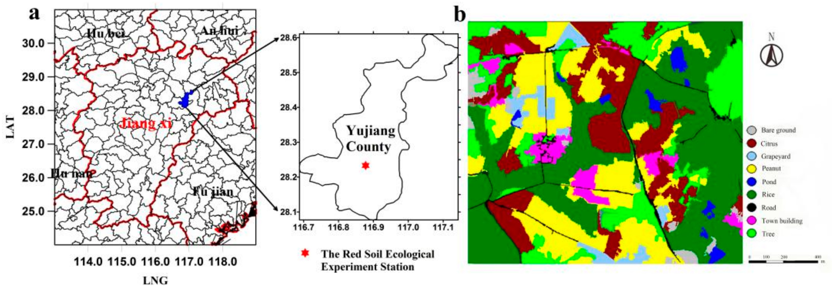
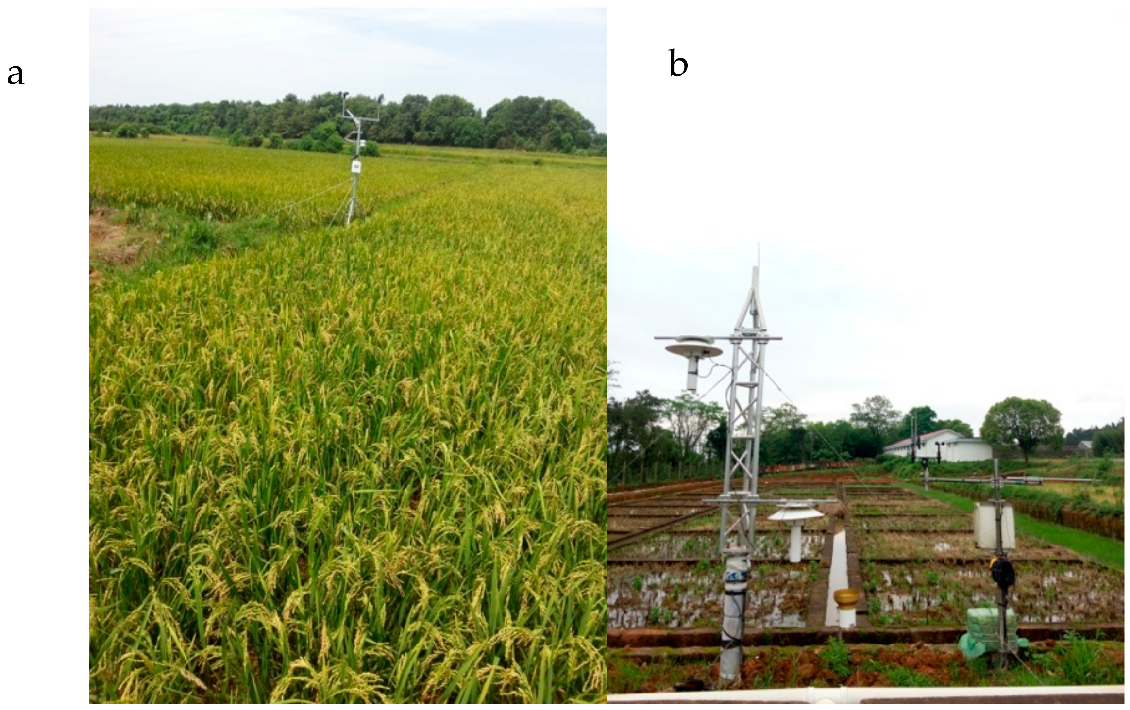
2.1. Experimental Site and Data

The field experiment was conducted at the Red Soil Ecological Experiment Station (116.89° E, 28.22° N) of the Chinese Academy of Sciences, located in Yujiang County, Jiangxi Province (Figure 1a) during 2014 and 2015. It has a subtropical monsoon climate with high temperatures and high humidity, characterized by abundant rainfall, ample light and distinct seasons. The annual average precipitation is 1794.7 mm, and the annual average water surface evaporation is 1229.1 mm. However, the seasonal distribution is uneven, and the rainy season (April to June) accounts for about 50% of the annual precipitation. The main soil parent material in the middle plain is Cretaceous red sandstone, Quaternary sub-sand and sand pebbles. The soil is divided into red soil, paddy soil and tidal soil according to the soil category. Red soil and paddy soil account for 48.97% and 45.30%, respectively. The farmland investigated in this study is referred to as the third field of Liujia reclamation farmland. The farmland area is about 100 ha, and the altitude is 40–54 m with 6–10 degree slope. The farmland was reclaimed in the 1980s. There were many dry crops on the outside of the farmland, such as peanut and citrus. The paddy fields were basically located in the middle. The underlying surface of the three crops accounted for 90% of the area of the entire research farmland (Figure 1b).

The atmospheric forcing data for SiB2 were obtained with fast-response sensors of automatic weather stations, which included radiation components, air temperature, humidity, wind speed, and precipitation, along with soil temperature and moisture content (Figure 2a). The radiometers (CNR-1, Kipp & Zonen, Delft, Netherland), which can measure downward shortwave/longwave and upward shortwave/longwave radiation separately, were installed at 2.2 m above the ground. The calculations of longwave radiation components were corrected as a thermal effect caused by instrument heating. Observations of water temperature in irrigated paddy field were carried out in the irrigated paddy field located within the site from July to October 2015. The inlet water temperature, outlet water temperature and water temperature were recorded by temperature sensor (HOBO U23, Onset, MA, USA, ±0.21 °C). These data were obtained every 30 min. All instruments were calibrated before the observations were made.

Fluxes of sensible heat (H) and latent heat (LE) were measured by the Bowen ratio energy balance system installed in a paddy field in the research farmland (Figure 2b). The system consists of two layers of high-accuracy temperature and humidity sensors, a net radiation sensor, a soil heat flux plate, solar power supply equipment, a waterproof tank, and data collectors (CR1000, Campbell, CA, USA). Temperature and humidity sensors (HC2S3, Campbell, CA, USA) had high measurement accuracy (±0.1 °C, ±0.8% RH, Standard conditions at 23 °C). The upper layer sensor was installed 3 m above ground and the lower layer sensor was installed 1.5 m above ground. Net radiation was measured using a NR-Lite net radiation sensor (Kipp & Zonen, Delft, The Netherland) installed 2.0 m above ground. Two soil heat flux plates (Hukseflux, HFP01, Delft, The Netherland) were buried 5 cm below the soil surface. Heat storage from the ground surface to 0.05 m depth was calculated from soil temperatures (at five depths and four locations) and their volumetric soil water contents. The system calculates the Bowen ratio by measuring the temperature gradient and water vapor pressure gradient between two layers, and then obtaining the latent heat flux and sensible heat flux according to the energy balance Equation as described below.

2.2. Bowen Ratio-Energy Balance Method

The principle of the Bowen ratio-energy balance method is the basis for calculating the energy balance of farmland. It is based on the theory of near-surface gradient diffusion and the energy balance equation of the underlying surface [24].

The Bowen ratio is defined as:

$$\beta =\frac{H}{\lambda E}$$

(1)

It also can be represented as the temperature and humidity gradient between different heights:

$$\beta =\frac{C_p{K}_h\frac{\partial T}{\partial Z}}{\lambda K_w\left(\frac{0.622}{P}\right)\frac{\partial e}{\partial Z}}$$

(2)

where ρ is air density (kg/m³); C_p is specific heat at constant pressure (usually $1004 \mathrm{J}·{\mathrm{kg}}^{-1}·{\mathrm{k}}^{-1}$); P is atmospheric pressure (hpa); K_h and K_w are thermal diffusion coefficient and water vapor diffusion coefficient, respectively (${\mathrm{m}}^2·{\mathrm{S}}^{-1}$); and T and e are air temperature (°C) and water vapor pressure (hpa), respectively. It is assumed that the thermal diffusion coefficient K_h is equal to water vapor diffusion coefficient K_w; then, Bowen ratio can be simplified to express as:

$$\beta =\gamma \Delta T/\Delta e$$

(3)

$$\lambda ET=\left(Rn-G\right)/\left(1+\beta \right)$$

(4)

$$H=\left(Rn-G\right)·\beta /\left(1+\beta \right)$$

(5)

where γ is psychrometric constant (0.667 hpa·°C⁻¹), ΔT is the air temperature difference at two heights, and Δe is the water vapor pressure difference at two heights. Using the calculated Bowen ratio, observed net radiation and soil heat flux, combined with the energy balance equation, we can finally obtain the sensible heat and latent heat flux (Equations (4) and (5)).

2.3. SiB2 Model

2.3.1. Overview of the SiB2 Model

The SiB2 model is a parameterization scheme to describe the exchange process of the land and atmosphere in which a set of physically-based Equations and parameters describe the turbulent transfer of heat and mass in the vegetation canopy [25,26]. The structure of the SiB2 model consists of atmospheric boundary conditions; morphological, physiological, and physical parameters; prognostic variables; and the governing equations. The SiB2 model describes net radiation, momentum, sensible heat and latent heat flux with one canopy layer and three soil layers at the surface soil, root zone and deep soil layers. In addition, the SiB2 model includes a photosynthesis-conductance model to calculate the coupled transfer of CO₂ and water vapor and the use of satellite data to describe the vegetation phenology.

SiB2 has 11 prognostic physical state variables: three temperatures (canopy, T_c; surface soil, T_g; and deep soil, T_d); two interception water stores (canopy, M_cw; and surface soil, M_gw); two interception snow/ice stores (M_cs and M_gs); three soil moisture wetness stores (surface soil, W1; root zone, W2; and deep soil, W3); and one prognostic (time-stepped) value of canopy conductance (g_c). Each of the three temperatures changes as a function of the surface energy fluxes, which are formulated in terms of their potential differences divided by aerodynamic resistances.

Energy budget components are calculated according to the energy balance equation. The detailed equations to calculate sensible (H_c and H_g) and latent (LE_c and LE_g) heat fluxes were given in Tables 3 and 4 of Sellers et al. [25].

2.3.2. Main Parameter Settings in Red Soil Farmland

The SiB2 model incorporates a canopy photosynthesis conductance sub-model to simulate a more realistic vegetation physiological process. It requires soil and vegetation types. These include morphological properties (e.g., canopy structure, leaf dimension, soil layer depth, etc.) (

Table 1. Parameter setting for the SiB2 model at Red Soil Ecological Experiment Station. Data were from direct observation or calculation.

Parameter	Description	Units	Value	Parameter	Description	Units	Value
Z2	Canopy-top height	m	1.3	D1	Depth of surface soil layer	m	0.05
Z1	Canopy-base height	m	0.2	Zw	Wind observation height	m	2.5
Zc	Inflection height for leaf-area density	m	0.777	ZT	Air temperature and humidity observation height	m	2
Zs	Ground roughness length	m	0.083	LAI	Leaf area index	-	3.82, 4.12, 2.6
ll	Leaf length	m	0.6	Zw	Wind observation height	m	2.5
lw	Leaf width	m	0.015	Corb1	non-neutral correction for calculation of aerodynamic resistance	-	0.086
Dr	Root depth	m	0.25	Corb2	neutral value of rb*u2,	-	184.05
Ds	Soil depth	m	1	G1	Augmentation factor for momentum transfer coefficient	-	1.449
V	Vegetation cover	%	95.6,96.2,94.6	G2	Transition height factor for momentum transfercoefficient	-	0.764

Note: “-”denotes unit less.

); optical properties (e.g., reflectance and transmittance for live and dead vegetation leaves); and physiological properties, which are mainly connected with the functioning of the photosynthesis-conductance model. The vegetation on this red soil farmland in southern China was dominated by C3 short-grass species. Therefore, the category was defined as “agriculture/C3 grassland” in short vegetation (biome type 9) [26]. The values of leaf area index at the different stages, canopy greenness fraction, and vegetation cover fraction in the second growing period of rice were based on our field measurements (Table 1). We divided the whole growing period into three stages. Stage 1 was from 23 July to 31 August with a leaf area index of 3.82 and a vegetation cover fraction of 0.956. Stage 2 was from 1 to 30 September with a leaf area index of 4.12 and a vegetation cover fraction of 0.962. Stage 3 was from 1 October to 31 October with a leaf area index of 2.6 and a vegetation cover fraction of 0.946.

Based on our experiment and observations in 2015, top and bottom heights of the short-grass canopy were 1.3 m and 0.02 m, respectively. The changes in the associated aerodynamic parameters in the SiB2 model were also taken into consideration by re-computing canopy roughness length, zero plane displacement, and the resistance coefficients for bulk boundary layer C1 and ground to canopy air-space C2 (

Table 2. Configuration changes at different stages of rice.

Parameter	Description	Units	Value Stage 1; Stage 2; Stage 3
LT	Leaf-area index	-	3.82	4.12	2.6
V	Vegetation cover	%	95.6	96.2	94.6
Z0	Canopy roughness length	m	0.083	0.095	0.087
D	Canopy zero plane displacement	m	0.895	0.869	0.854
C1	Bulk boundary-layer resistance coefficient	(s m−1)	9.67	9.46	12.30
C2	Ground to canopy air-space resistance coefficient	(s m−1)	42.80	86.30	79.66

Note: “-” denotes unit less.

). The depth of total soil layer was 1 m according to maximum depth of our observation and three soil layers were defined as surface layer (D₁ = 0.05 m), root zone (D₂ = 0.15 m), and recharge zone (D₃ = 0.25 m) by actual measurement.

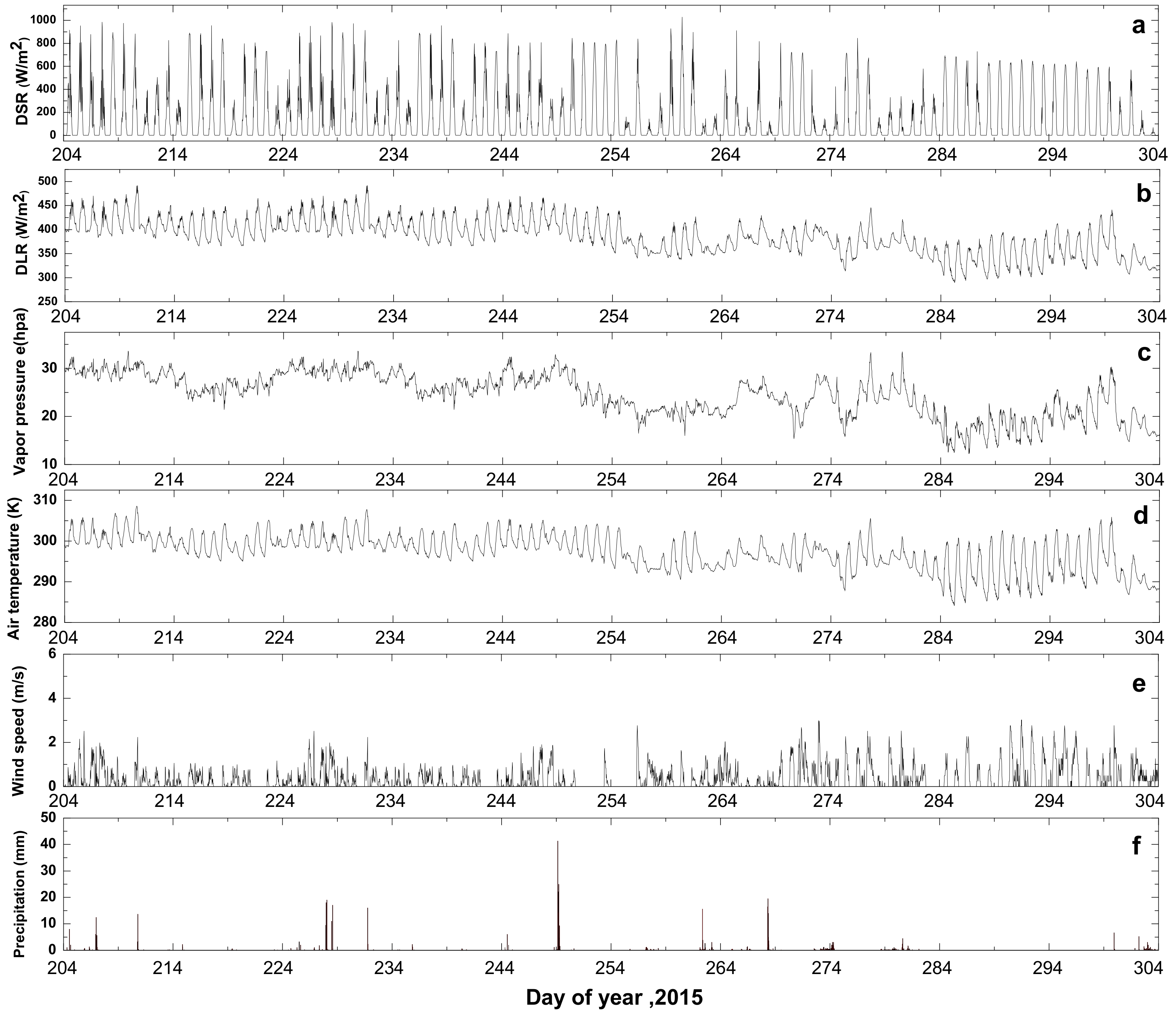
2.3.3. Driving Data for the SiB2 Model Used in this Study

The SiB2 model requires atmospheric driving data (as the model was used here in an off-line uncoupled fashion): downward shortwave radiation, downward longwave radiation, air temperature, vapor pressure, wind speed, and precipitation. These forcing data were measured with the automatic weather station instrument located inside the paddy field at the research farmland. The simulation period was from 23 July to 31 October, which encompassed summer and autumn in the red soil region of southern China in 2015 (Figure 3). As the summer monsoon progressed, forcing data at the early stage showed no significant variation. However, in autumn, when precipitation decreases in the middle of September (on around Day 256), the forcing data also varied. Radiation decreased throughout the rice growing season and the daily maximum value of DSR/DLR decreased from 984.6 Wm⁻²/491.6 Wm⁻² in August to 962.5 Wm⁻²/469.2 Wm⁻² in October. The decrease in vapor pressure was more obvious, at around 30 hpa in August, while the average in October was only 22.1 hpa. The daily air temperature range increased from 6.7 °C in August to 11.6 °C in October. There was no particular change in wind speed in the different stages of rice growth, with an average wind speed of about 0.3–0.4 m/s.

2.3.4. Initialization in the SiB2 Model

Table 3. Initial parameter used in this research.

Initial Parameter	Initial Value
Canopy temperature	300.6 K
Ground surface temperature	302.0 K
Deep soil temperature	302.5 K
Canopy air space temperature	300.6 K
Volumetric water content at soil surface layer	0.30
Volumetric water content at root zone	0.30
Volumetric water content at recharge zone	0.30

gives the initial conditions for SiB2. Initial temperatures of the canopy, canopy air space, surface soil, and deep soil, as well as soil wetness, were directly determined using our field observations at Red Soil Ecological Experiment Site. These values were obtained based on averages from two years of actual observation (2014 and 2015).

2.4. The Adjustment of the SiB2 Model for Paddy Fields in Southern China

Considering the irrigation activity of the southern paddy field during its growing season, parameter values cannot be adjusted to reflect the actual situation, and it is necessary to increase the water layer calculation in the original SiB2 model. Here, we assumed that short wave radiation could be completely absorbed by the water layer, as the water body is usually very muddy in irrigated farmland. At the same time, radiation decreases with the exponential change in crop canopy. Kim et al. [23] provided the calculation method for the crop water layer. The calculation of the water layer and soil layer of irrigated farmland can be expressed in the following equations:

$$C_w\frac{\partial T_w}{\partial t}=R{n}_w-H_w-L{e}_w-\lambda \frac{T_w-T_a}{(D_w+D_g)/2}$$

(6)

$$C_g\frac{\partial T_g}{\partial t}=R{n}_g+\lambda \frac{T_w-T_g}{(D_w+D_g)/2}-\frac{2\pi C_d}{\tau }(T_g-T_d)$$

(7)

where C_w and C_g represent effective heat capacity ($\mathrm{J}·{\mathrm{m}}^{-2}·{\mathrm{K}}^{-1}$) for water and soil, respectively; and T_w, T_g, and T_a represent the temperatures of water, soil, and air, respectively. D_w and D_g are the depth of water and soil. τ means day length(s). T_d is the temperature of the deep soil. The specific calculations were provided in Equations (3)–(7) of Kim et al. [23]. In the case of irrigation, the traditional surface energy balance should also increase the water heat storage (W) in addition to the soil heat flux (G).

However, in Kim’s method, the temperature change due to water inflow/outflow was negligible. In our experiment, a new heat item (Q_f) was added to Equation (6) to describe the heat change due to water flow:

$$Q_f=C_w{\rho }_{w}V(T_{out}-T_{in})$$

(8)

where V means water flow velocity (m/s) and T_out and T_in represent outflow/inflow water temperature.

2.5. Statistical Analysis and Sensitivity Analysis

We used the traditional statistical analysis index to evaluate the accuracy of the model. In this study, the single-factor sensitivity analysis method was used to discriminate the influence of different parameters on the result of the model. The following comparison statistics were calculated:

Bias:

$$Bias={\displaystyle \sum _{i=1}^n\frac{M_i-O_i}{n}}$$

(9)

where M_i is the value modeled by the SiB₂ model, O_i is the observed values, and n is the total number of data points (n = 4848 in this study). If the value of bias is small, the simulation will be close to the observed value.

Root-mean-square Error of the Simulation (RMSE):

$$RMSE=\sqrt{\frac{{\displaystyle \sum _{i=1}^n{(M_i-O_i)}^2}}{n}}$$

(10)

RMSE indicates the discrete situation between the simulated value and the observed value.

Sensitivity of the Variable y to the Single Variable x is defined as a partial derivative $\frac{\partial y}{\partial x}$, and can be represented as:

$$S(x_i)=\frac{\partial y}{\partial x}=\frac{\Delta y}{\Delta x_i}$$

(11)

In this study, we selected the main forcing meteorological factors (downward short-wave radiation, downward long-wave radiation, vapor pressure, air temperature, and wind speed), surface soil moisture (Ws), and the resistance coefficients (C1 and C2) that have a direct impact on the estimation of latent heat flux and sensible heat flux, to analyze the influence of these parameters on the result of the model.

3. Results and Discussion

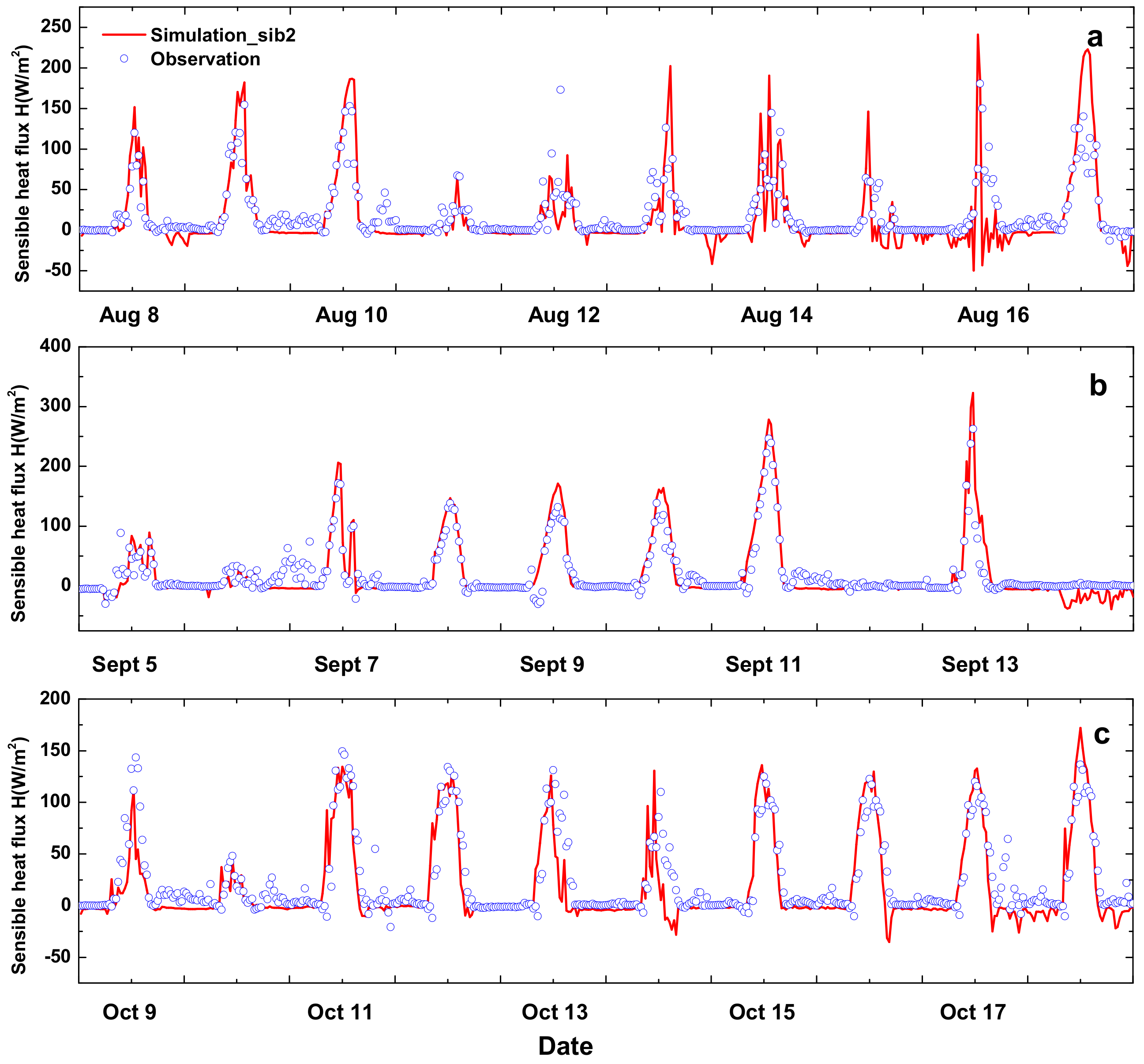
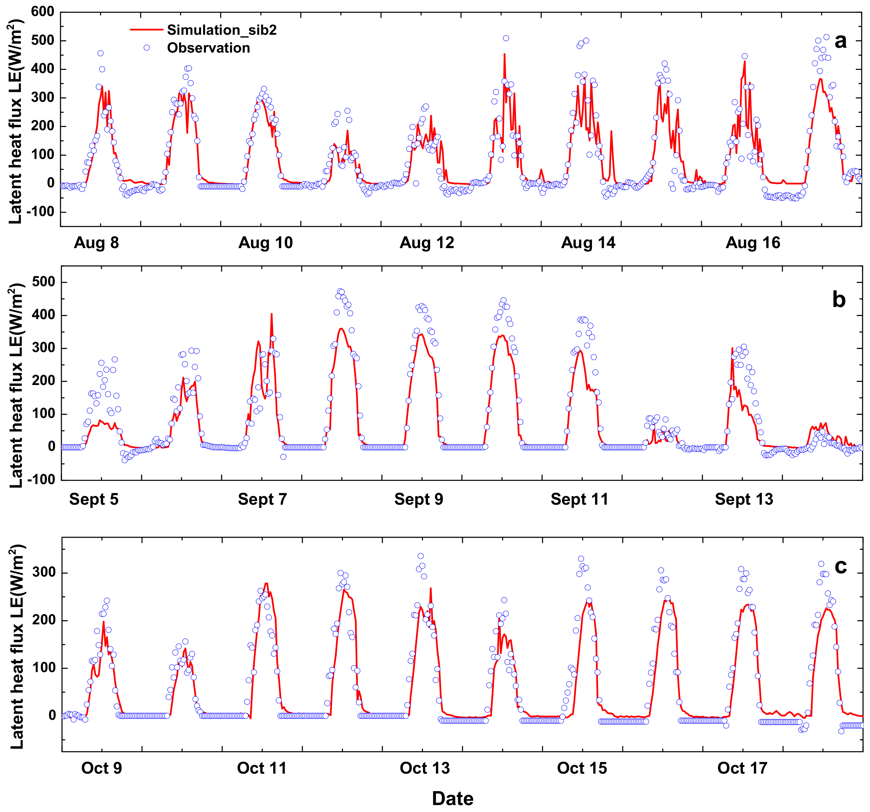
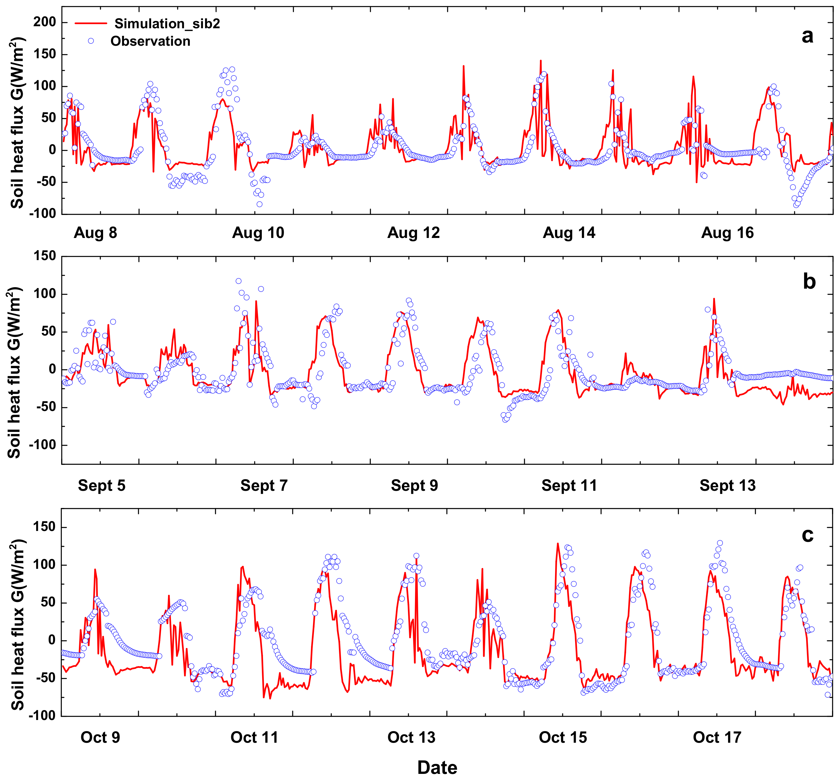
3.1. Comparison of Measured and Modeled Surface Energy Flux

The whole research period was divided into three stages based on the different growth stages of late rice in 2015 as rice is the most representative crop of the farmland region, so that the parameters settings of SiB2 would be more accurate and appropriate. To reveal the characteristics of the energy balance component in typical red soil farmland of southern China and evaluate the accuracy of SiB2 simulation more effectively, we selected a ten-day period in each stage to analyze diurnal changes: (1): 8–17 August, the tillering stage of late rice; (2): 5–14 September, the booting stage of late rice; and (3): 9–18 October, the maturation stage of late rice.

Net radiation was derived from the four components of the radiation budget: upward and downward components of shortwave and longwave radiation. The first two downward components were given as forcing data (Figure 3), whereas SiB2 simulated the latter two upward components. Consequently, any errors in outgoing short-wave radiation and outgoing long-wave radiation would result in proportional errors in R_n simulation.

Figure 4 shows the Rn simulated using the SiB2 model and measured using the Bowen ratio-energy balance system at the different growth stages of rice. In general, the SiB2 model captured the peak and the diurnal pattern of Rn. On some days with heavy rain (e.g., on 5 and 6 September, average daily precipitation reached 65 mm), the SiB2 model underestimated Rn slightly.

The modeled and measured values of H and LE at the different growth stages of rice are shown in Figure 5 and Figure 6. Compared to Rn, H had an irregular change trend throughout the study period. The peak value of LE was closer to Rn. The changing trend of LE was consistent with Rn during the study period, as LE was the most important part of the energy distribution of Rn.

The SiB2 model was also reasonably able to capture the peak and diurnal pattern of H, especially at Stages 2 and 3. At Stage 1, the SiB2 model overestimated H. The possible reason for this is that heat exchange in SiB2 needs to be carried out with a relatively uniform underlying surface, in which case the setting of such parameters and the output of results can be more stable. At Stage 1, however, the vegetation coverage was low and soil surface was complex. The SiB2 model underestimated LE in the daytime at different stages of the research period, but the night performance was still good. The soil moisture sensors of our experimental observation were not installed directly inside the paddy field, resulting in the surface soil moisture parameters set in SiB2 to be less than the actual value. Additionally, the influence of irrigation was not considered in the original SiB2 model, so the existence of the surface water layer was neglected. These might be the reasons that LE was underestimated.

Figure 7 shows the G simulated using the SiB2 model and measured using the Bowen ratio-energy balance system at the different growth stages of rice. SiB2 generated consistent temporal variations in G with observation at all stages. It is worth mentioning that G returned more negative values in October, which indicated that soil released heat into the atmosphere at this stage and the deep soil temperature was higher than at the surface layer. At the last stage of rice growth, due to the simulated value of the surface soil temperature (Tg) being more than the actual value, modeled G was significantly less than the measured value (

Table 4. Computed Bias, RMSE (W m⁻²) of energy balance components at three stages and the whole period.

	Stage 1 23–31 July		Stage 2 1–30 September		Stage 3 1–31 October		Whole Growth Stage
	Bias	RMSE	Bias	RMSE	Bias	RMSE	Bias	RMSE
Rn	1.52	63.5	0.62	54.2	−0.92	56.15	0.71	58.97
H	4.52	46.3	4.23	26.3	2.34	20.4	3.88	30.71
LE	−7.83	48.3	−6.57	56.1	−3.56	62.4	−6.35	46.4
G	−1.2	34.6	−2.64	23.4	−3.01	34.5	−2.32	29.5

), especially at nighttime.

It was obvious that SiB2 generated consistent temporal variations in Rn, H, LE, and G. The squared correlation coefficients were 0.87, 0.58, 0.80, and 0.33, respectively. Scatter plots of the modeled Rn, H, LE and G values against measured values are given in Figure 8, which show that SiB2 overestimated Rn and H by 0.07% and 16.9%, respectively, and underestimated LE and G by 16.0% and 7.6%, respectively. Table 4 presents two statistical indices, Bias, and RMSE for the three stages (n = 1920, 1440, 1488) and the whole research period (n = 4848). There was a slight positive bias of about 1.08 Wm⁻² in Rn when RSME was 58.97 Wm⁻² throughout the period. This indicates that the average values of the simulation were consistent with the measured values, but there were still a few outlier values between the model and observation. The negative bias in LE and G suggests that the model tended to underestimate these energy components. The simulation bias of H and LE decreased gradually during the research period, mainly due to the increase in vegetation coverage during the last growth stage of rice along with the reduction in surface irrigation activities, which made SiB2 perform better (Figure 5 and Figure 6, and Table 4). Modeling the energy balance component using the parameter scheme we set at Red Soil Ecological Experiment Station can be adapted to the situation in the red soil farmland region of southern China, but it still has some issues when it comes to energy distribution.

3.2. Sensitivity Analysis of Energy Flux

To understand the influence of model parameters on simulation and to find a more appropriate parameterizing scheme, the modeled energy fluxes (Rn, H, and LE) at Stage 1 were assessed via sensitivity analysis. Moreover, due to the uncertainty of the meteorological observations, which can also affect the simulation results, it is reasonable to carry out sensitivity analysis of the primary meteorological input factors. Here, we selected five meteorological factors (i.e., DSR, DLR, u, Ta, and e) from the driving data, two resistance parameters (i.e., C1 and C2), and the soil moisture parameter from the key computing process of LE and H as the adjustable factors.

As important aerodynamic parameters in SiB₂, C1 was the bulk canopy (vegetation) to canopy-air resistance coefficient, and C2 was the ground to canopy-air resistance coefficient. Thus, C1 determined energy and water flux movement between the leaf and the canopy air, and C2 determined flux exchanges between the ground and the canopy air. It is necessary to study the effect of these changes on surface energy flux. The range of the adjustment is listed in

Table 5. Range of parameters in sensitivity experiments.

Parameter	Initial Value	Value in Sensitivity Test
DSL	based on driving data	±10%, ±15%, ±20%,
DLR
Ta
e
u
C1	9.67	+10, +20, +30
C2	42.8	+10, +20, +30
Ws	0.3	0.5, 0.7, 0.9

. The reasonable range of the aerodynamic resistance coefficient and stomatal resistance coefficient in the model are 0–200 and 40–200 s/m, respectively. Thus, the parameters used in our sensitivity experiments are reasonable. Considering the uncertainty in soil surface moisture (Ws) observation and its key role in crop transpiration, we took the sensitivity test for soil moisture parameter by selecting three levels above the observation value (0.5, 0.7, and 0.9).

Through sensitivity analysis of the driving meteorological factors, we found that the modeled energy flux had higher sensitivity to downward short-wave radiation (DSR), downward long-wave radiation (DLR) and wind speed (u), of which average sensitivity could exceed 0.5 (

Table 6. Sensitivity of energy fluxes to adjustable driving data (Only the sensitivity more than 0.1 was listed).

Factor		Rn			LE			H
		Bias	RMSE	S(i)	Bias	RMSE	S(i)	Bias	RMSE	S(i)
DSR	+10%	11.1	18.3	0.70	2.6	8.6	0.17	8.3	16.5	0.55
	+15%	16.7	19.6	0.72	3.5	8.9	0.11	12.6	18.5	0.56
	+20%	20.6	20.5	0.73	3.4	7.5	0.13	16.4	20.3	0.52
	−10%	−10.8	17.6	0.68	−4.2	10.6	0.21	−7.9	15.2	0.51
	−15%	−15.3	18.8	0.69	−5.1	9.6	0.16	−13.4	19.5	0.57
	−20%	−21.6	22.4	0.73	−5.6	11.5	0.14	−17.6	22.6	0.52
DLR	+10%	31.5	25.6	0.79	7.2	10.3	0.18	23.1	22.3	0.52
	+15%	49.6	28.4	0.81	8.3	11.5	0.14	40.6	25.6	0.65
	+20%	67.1	29.4	0.82	8.5	11.7	0.10	56.8	28.2	0.68
	−10%	−30.1	22.4	0.81	−10.2	15.3	0.21	−21.4	21.5	0.51
	−15%	−44.9	25.2	0.78	−18.3	16.2	0.22	−16.2	18.5	0.26
	−20%	−59.5	28.3	0.80	−22.5	20.4	0.23	−23.4	22.4	0.28
u	+10%	-	-	-	1.22	7.5	0.45	3.42	9.6	0.65
	+15%	-	-	-	1.34	8.36	0.31	5.2	10.6	0.76
	+20%	-	-	-	2.42	12.5	0.36	6.4	12.5	0.72
	−10%	-	-	-	−0.86	6.5	0.32	−4.2	13.5	0.73
	−15%	-	-	-	−1.02	7.4	0.26	−6.2	14.4	0.65
	−20%	-	-	-	−1.14	10.5	0.16	−8.1	18.3	0.84

). As DSR and DLR were input items in the process of Rn simulation, they had a positive correlation with the simulated Rn and H. However, LE was not greatly affected by them. Bias was only 2.6 and 7.2 Wm⁻² and Sensitivity was only 0.17 and 0.18, while DSR and DLR increased by 10%. The effect of wind speed on Rn was quite small, but it had great influence on the H. This is because the increase in wind speed results in a reduction of the aerodynamic impedance, which is beneficial to the heat exchange between the land surface and the atmosphere.

In the two resistance coefficients, C1 had prominent positive correlation with the simulated H and negative correlation with the simulated LE (

Table 7. Sensitivity of energy fluxes to resistance coefficient (C1, C2) and soil surface humidity (Ws).

Factor		Rn			LE			H
		Bias	RMSE	S(i)	Bias	RMSE	S(i)	Bias	RMSE	S(i)
C1	+10	-	-	-	−10.9	15.7	−1.09	8.9	14.5	0.89
	+20	-	-	-	−16.4	18.2	−0.94	15.3	17.2	0.65
	+30	-	-	-	−20.6	20.1	−0.82	16.7	19.6	0.58
C2	+10	-	-	-	−4.1	8.6	−0.14	−7.3	15.2	−0.67
	+20	-	-	-	−5.1	8.9	−0.12	−11.2	19.5	−0.56
	+30	-	-	-	−5.3	9.5	−0.12	−13.6	22.6	−0.54
Ws	0.5	-	-	-	−1.8	13.4	6.9	1.7	12.8	6.5
	0.7	-	-	-	−0.3	1.2	5.4	0.3	0.8	5.0
	0.9	-	-	-	0.7	15.4	5.1	−0.6	13.5	−4.3

). The change in C2 cannot produce large fluctuations in LE, but it has a negative correlation with H. Soil surface moisture (Ws) had an obvious positive correlation with LE, and the low value of soil moisture parameters would directly lead to the underestimation of LE and overestimation of H.

The different land surface modes or input data in different sites used in sensitivity experiments can sometimes provide different results. However, the results are not the same for different underlying surfaces or in different seasons [27,28,29,30]. Therefore, the results of the sensitivity analysis in this study are suitable for the red soil farmland region of southern China.

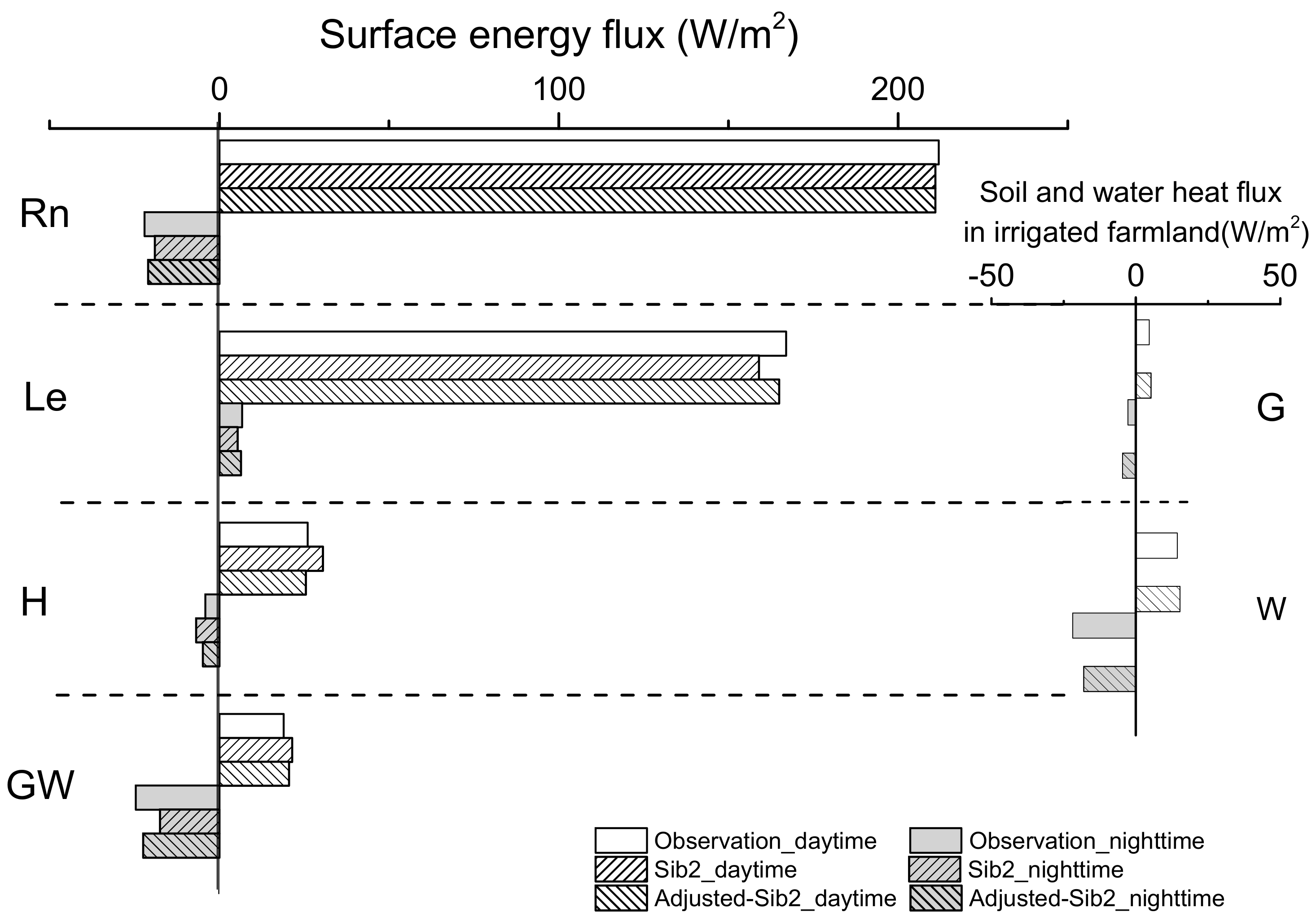
3.3. Results of the Adjusted SiB2 Model

According to the results of sensitivity analysis,

Table 8. Aerodynamic parameters and soil humidity parameter used in original SiB2 and adjusted SiB2.

Adjusted Parameter	Definition	Units	Original Value	Adjusted Value (Non-Irrigation)	Adjusted Value (Irrigation)
C1	Bulk boundary-layer resistance coefficient	-	9.67	4.67	4.67
C2	Ground to canopy air-space resistance coefficient	-	42.8	72.8	72.8
Ws	Volumetric water content at soil surface layer	%	30	40	48

Note: “-” denotes unit less.

gives adjusted parameters for SiB2 in different irrigation conditions. C1 and C2 were reset as 4.67 and 72.8, respectively, because they were the most suitable parameter values used in the model to match the simulated values with observation based on the results of repeated tests. In the test, C1 and C2 were set at four levels, respectively (C1: 2.67, 4.67, 6.67, and 8.67; and C2: 52.8, 62.8, 72.8, and 82.8), in which C1 was less than the initial value, and C2 was greater than the initial value. We evaluated simulated flux results with different combinations, and then determined the scheme. The surface soil moisture was increased slightly in order to better reflect the actual conditions. Although our soil observation site was next to the rice field, soil moisture was still lower than the average in the paddy field. For paddy field during irrigation, we used saturated soil moisture content measured in the paddy field (48%) as the surface soil moisture parameter in the model. The first stage was divided into two cases: (1) irrigation, using the improved SiB2 model to simulate surface energy flux combined with the adjusted parameters (Irrigation); and (2) non-irrigation, using the original SiB2 model combined with the adjusted parameter (Non-irrigation) for simulation.

Figure 9 illustrates the mean surface energy balance components from observation and from two simulations. The result of Rn was consistent with the previous results, and the results of the two simulations were both very close to the results of observation. Simulated GW (soil and water heat flux), and W (water heat flux) using the adjusted SiB2 model were in good agreement with the observation results. It could be seen that the water environment of the paddy field after adjustment was more consistent with the actual situation. The adjusted SiB2 model had significant improvement in the simulation of H and LE both in the daytime and nighttime. The original SiB2 had a high underestimation of LE and a high overestimation of H. After adjusting and improving SiB2, the mean daytime error of LE decreased from 7.8 Wm⁻² to 2.3 Wm⁻², and the bias of H decreased from 4.5 Wm⁻² to 1.5 Wm⁻² in Stage 1.

4. Conclusions and Discussion

Modeling land surface processes plays an important role in understanding the interaction between the land surface and the atmosphere [31,32,33,34]. The energy and water balance should always be held at the land surface, and it should impact all-scale models [35,36,37,38]. In this study, we collected and processed the measured data from the low-hilly red soil farmland region of southern China at The Red Soil Ecological Experiment Station in 2015. We also listed our parameter settings and adjustments for the SiB2 model at the Red Soil site and reported modeled results of energy budget components from 23 July to 31 October 2015.

Daily patterns of net radiation (Rn), sensible heat flux (H), latent heat flux (LE), and soil heat flux (G) modeled using SiB2 are consistent with direct measurements. Similar to direct measurements, the modeled daily patterns of H, LE and G followed that of Rn. We compared SiB2 with the Bowen ratio energy balance algorithm of sensible and latent heat fluxes by using the data collected in the red soil farmland region of southern China. We found, on average, that SiB2 overestimated H by 16.9% and underestimated LE by 16.0%. Rn and G were reasonably estimated.

The sensitivity analysis of Rn, H, and LE modeled in SiB2 indicated that downward shortwave radiation (DSR) and downward longwave radiation (DLR) have a significant influence on the simulation of Rn. In driving data, DSR, DLR and wind speed (u) were the main factors that can cause distinct changes in H. In the two resistance coefficients, an increase in C1 can cause an increase in H and a prominent decrease in LE. A change in C2 cannot produce large fluctuations in LE, but had a negative correlation with H.

The errors between simulated land surface energy components using SiB2 and observation also exist in similar studies. In the Global Energy and Water Cycle Experiment (GEWEX) Asian Monsoon Experiment (GAME)-Tibet project, Rn was underestimated by 11%, while H, LE, and G were overestimated by 8%, 3%, and 13%, respectively, using SiB2 [2]. Li et al. [3] modeled energy components for alpine meadows in the upper reaches of the Heihe River, and their results showed that H was overestimated by 28% and LE was underestimated by 12%. After adjusting the optimum growth temperature to 288 K based on the average daily temperature during their study period (default value is 298 K), the biases in H, LE and G were reduced to a large extent (to less than 7% bias). Unfortunately, our study found that this method is not applicable in the southern China red soil region, as the default optimum growth temperature in SiB2 is very close to the average temperature in our study area (about 300 K from July to October), so the effect of the change in optimum growth temperature on the final simulation result is quite small.

According to the results of sensitivity analysis, the uncertainty of the H and LE simulation may come from two radiations and wind speed input or resistance parameters C1/C2 and soil surface humidity parameter (Ws). Parameters C1 and C2 were reset to 4.67 and 72.8, respectively. Considering the influence of irrigated paddy fields, the original SiB2 model was adjusted with changes to the parameters C1, C2, and Ws. Kim et al. [23] also considered the influence of surface water on the simulation. It was found that the bias of H (modeled by SiB2-Paddy) was reduced significantly compared with the original model, but there was no obvious change in LE. In our results, the simulation biases of both H and LE were significantly reduced; this is partly because we added a new heat item in the irrigation module that was suited to the real situation, and the adjustment of parameters in SiB2 was appropriate. The results illustrate that the improved method can be better applied to southern farmland in China.

This study is only the beginning of land surface simulation in the red soil region of southern China. In the next study, we will configure the parameters of several sites in the red soil region of southern China and use satellite data to realize an accurate land surface process simulation at the regional scale. Due to the lack of simulation inside the vegetation canopy in traditional land surface process models, energy exchange in the canopy cannot be well explained [39]. Through the application of land surface models combined with principles of micrometeorology and plant physiology, we will try to improve the SiB2 model and supplement simulations of energy exchange at different heights in the vegetation canopy.

References

1. Defries, R.S.; Bounoua, L.; Collatz, G.J. Human modification of the landscape and surface climate in the next fifty years. Glob. Chang. Biol. 2002, 8, 438–458. [Google Scholar] [CrossRef]
2. Gao, Z.; Chae, N.; Kim, J.; Hong, J.; Choi, T.; Lee, H. Modeling of surface energy partitioning, surface temperature, and soil wetness in the Tibetan prairie using the Simple Biosphere Model 2 (SiB2). J. Geophys. Res. Atmos. 2004, 109, D06102. [Google Scholar] [CrossRef]
3. Li, Y.; Sun, R.; Liu, S. Vegetation physiological parameter setting in the simple biosphere model 2 (SiB2) for alpine meadows in the upper reaches of Heihe river. Sci. Chin. Earth Sci. 2015, 58, 755–769. [Google Scholar] [CrossRef]
4. Niraula, R.; Meixner, T.; Ajami, H.; Rodell, M.; Gochis, D.; Castro, C.L. Comparing potential recharge estimates from three land surface models across the Western US. J. Hydrol. 2017, 545, 410–423. [Google Scholar] [CrossRef] [PubMed]
5. Rowntree, P.R. Atmospheric parameterization schemes for evaporation over land: Basic concepts and climate modeling aspects. In Land Surface Evaporation. Measurement and Parameterization; Springer: Berlin, Germany, 1991. [Google Scholar]
6. Dickinson, R.E.; Hendersin-Sellers, A.; Rosenzweig, C.; Sellers, P.J. Evapotranspiration models with canopy resistance for use in climate models: A review. Agric. For. Meteorol. 1991, 54, 373–388. [Google Scholar] [CrossRef]
7. Zhang, X.; Gao, Z.Q.; Wei, D.P. The sensitivity of ground surface temperature prediction to soil thermal properties using the simple biosphere model (SiB2). Adv. Atmos. Sci. 2012, 29, 623–634. [Google Scholar] [CrossRef]
8. Chen, Y.; Yang, K.; Zhou, D.G.; Qin, J.; Guo, X.F. Improving the Noah land surface model in arid regions with an appropriate parameterization of the thermal roughness length. J. Hydrometeorol. 2010, 11, 995–1006. [Google Scholar] [CrossRef]
9. Larsen, M.A.D.; Refsgaard, J.C.; Jensen, K.H.; Butts, M.B.; Stisen, S.; Mollerup, M. Calibration of a distributed hydrology and land surface model using energy flux measurements. Agric. For. Meteorol. 2016, 217, 74–88. [Google Scholar] [CrossRef] [Green Version]
10. Zhang, B.; Kang, S.; Li, F.; Lu, Z. Comparison of three evapotranspiration models to Bowen ratio-energy balance method for a vineyard in an arid desert region of Northwest China. Agric. For. Meteorol. 2008, 148, 1629–1640. [Google Scholar] [CrossRef]
11. Rannik, Ü.; Peltola, O.; Mammarella, I. Random uncertainties of flux measurements by the eddy covariance technique. Atmos. Meas. Tech. 2016, 9, 1–31. [Google Scholar] [CrossRef]
12. Li, G.; Zhang, F.; Jing, Y.; Liu, Y.; Sun, G. Response of evapotranspiration to changes in land use and land cover and climate in China during 2001–2013. Sci. Total Environ. 2017, 256, 596–597. [Google Scholar] [CrossRef]
13. Li, X.; Cheng, G.; Liu, S.; Xiao, Q.; Ma, M.; Jin, R.; Che, T.; Liu, Q.; Wang, W.; Qi, Y.; et al. Heihe watershed allied telemetry experimental research (HIWATER): Scientific objectives and experimental design. Bull. Am. Meteorol. Soc. 2013, 94, 1145–1160. [Google Scholar] [CrossRef]
14. Ma, Y.M.; Kang, S.C.; Zhu, L.P.; Xu, B.Q.; Tian, L.D.; Yao, T.D. Tibetan observation and research platform atmosphere-land interaction over a heterogeneous landscape. Bull. Am. Meteorol. Soc. 2008, 89, 1487–1492. [Google Scholar]
15. Koike, T. The coordinated enhanced observing period—An initial step for integrated global water cycle observation. WMO Bull. 2004, 53, 115–121. [Google Scholar]
16. Xu, X.; Zhang, R.; Koike, T.; Lu, C.; Shi, X.; Zhang, S.; Bian, L.; Cheng, X.; Li, P.; Ding, G. A new integrated observational system over the Tibetan plateau. Bull. Am. Meteorol. Soc. 2008, 89, 1492–1496. [Google Scholar]
17. Ping, Z.; Bounoua, L.; Thome, K.; Wolfe, R.; Imhoff, M. Modeling surface climate in U.S. cities using simple biosphere model SiB2. Can. J. Remote Sens. 2015, 41, 525–535. [Google Scholar]
18. Song, Y.; Ma, M.; Li, X.; Wang, X. Scaling from instantaneous remote-sensing-based latent heat flux to daytime integrated value with the help of SiB2. In Remote Sensing for Agriculture, Ecosystems, and Hydrology XIII; International Society for Optics and Photonics: Bellingham, WA, USA, 2011. [Google Scholar]
19. Qiu, R.; Du, T.; Kang, S.; Chen, R.; Wu, L. Assessing the SIMDualKc model for estimating evapotranspiration of hot pepper grown in a solar greenhouse in Northwest China. Agric. Syst. 2015, 138, 1–9. [Google Scholar] [CrossRef]
20. Sridhar, V.; Elliott, R.L.; Chen, F.; Brotzge, J.A. Validation of the NOAH-OSU land surface model using surface flux measurements in Oklahoma. J. Geophys. Res. 2002, 107, 4418–4436. [Google Scholar] [CrossRef]
21. Yan, X.D.; Hui-Yang, L.I.; Liu, F.; Gao, Z.Q.; Liu, H.Z. Modeling of surface flux in Tongyu using the simple biosphere model 2 (SiB2). J. For. Res. 2010, 21, 183–188. [Google Scholar] [CrossRef]
22. Liu, F.; Tao, F.; Xiao, D.; Zhang, S.; Wang, M.; Zhang, H. Influence of land use change on surface energy balance and climate: Results from SiB2 model simulation. Prog. Geogr. 2014, 33, 815–824. [Google Scholar]
23. Kim, W.; Arai, T.; Kanae, S.; Oki, T.; Musiake, K. Application of the simple biosphere model (SiB2) to a paddy field for a period of growing season in game-tropics. J. Meteorol. Soc. Jpn. 2001, 79, 387–400. [Google Scholar] [CrossRef]
24. Todd, R.W.; Evett, S.R.; Howell, T.A. The bowen ratio-energy balance method for estimating latent heat flux of irrigated alfalfa evaluated in a semi-arid, advective environment. Agric. For. Meteor. 2000, 103, 335–348. [Google Scholar] [CrossRef]
25. Sellers, P.J.; Randall, D.A.; Collatz, G.J.; Berry, J.A.; Field, C.B.; Dazlich, D.A.; Zhang, C.; Collelo, G.D.; Bounoua, L. A revised land surface parameterization (SiB2) for atmospheric GCMs. Part I: Model Formulation. J. Clim. 1996, 9, 676–705. [Google Scholar] [CrossRef]
26. Sellers, P.J.; Los, S.O.; Tucker, C.J.; Justice, C.O.; Dazlich, D.A.; Collatz, G.J.; Randall, D.A. A revised land surface parameterization (SiB2) for atmospheric GCMs. Part II: The generation of global fields of terrestrial biophysical parameters from satellite data. J. Clim. 1996, 9, 706–737. [Google Scholar] [CrossRef]
27. Lindroth, R.L.; Kinney, K.K.; Platz, C.L. Responses of deciduous trees to elevated atmospheric CO2: Productivity, phytochemistry, and insect performance. Ecology 1993, 74, 763–777. [Google Scholar] [CrossRef]
28. Randall, D.A.; Dazlich, D.A.; Zhang, C.; Denning, A.S.; Sellers, P.J.; Tucker, C.J.; Bounoua, L.; Berry, J.A.; Collatz, G.J.; Field, C.B.; et al. A revised land surface parameterization (SiB2) for atmospheric GCMs. Part III: The Greening of the Colorado State University General Circulation Model. J. Clim. 1996, 9, 738–763. [Google Scholar] [CrossRef]
29. Chen, L.; Reiter, X.E.; Feng, Z.Q. The atmospheric heat source over the Tibetan plateau: May–August 1979. Mon. Weather Rev. 1985, 113, 1771–1790. [Google Scholar] [CrossRef]
30. Tanaka, K.; Ishikawa, H.; Haysshi, T.; Tamagawa, I.; Ma, Y. Surface energy budget at Amdo on the Tibetan Plateau using GAME/Tibet IOP98 Data. J. Meteorol. Soc. Jpn. 2001, 79, 505–517. [Google Scholar] [CrossRef]
31. Chen, F.; Dudhia, J. Coupling an advanced land-surface/hydrology model with the Penn State-NCAR MM5 modeling system, part I, Model implementation and sensitivity. Mon. Weather Rev. 2001, 129, 569–582. [Google Scholar] [CrossRef]
32. Colello, G.D.; Grivet, C.; Sellers, P.J.; Berry, J.A. Modeling of energy, water, and CO2 flux in a temperate grassland ecosystem with SiB2: May–October 1987. J. Atmos. Sci. 2010, 55, 1141–1169. [Google Scholar] [CrossRef]
33. Bian, L.; Gao, Z.; Xu, Q.; Lu, L.; Chen, Y. Measurements of Turbulence Transfer in the Near Surface Layer over the Southeastern Tibetan Plateau. Bound. Layer Meteorol. 2002, 102, 281–300. [Google Scholar] [CrossRef]
34. Gao, Z.; Fan, X.; Bian, L. Analytical Solution to One-Dimensional Thermal Conduction-Convection in Soil. Soil Sci. 2003, 168, 99–106. [Google Scholar] [CrossRef]
35. Li, G.; Jing, Y.; Wu, Y.; Zhang, F. Improvement of Two Evapotranspiration Estimation Models Using a Linear Spectral Mixture Model over a Small Agricultural Watershed. Water 2018, 10, 474. [Google Scholar] [CrossRef]
36. Li, X.; Gao, Z.; Li, Y.; Tong, B. Comparison of sensible heat fluxes measured by a large aperture scintillometer and eddy covariance system over a heterogeneous farmland in East China. Atmosphere 2017, 8, 101. [Google Scholar] [CrossRef]
37. Li, X.; Li, X.; Li, Z.; Ma, M.; Wang, J.; Xiao, Q.; Liu, Q.; Che, T.; Chen, E.; Yan, G.; et al. Watershed allied telemetry experimental research. J. Geophys. Res. Atmos. 2009, 114, 2191–2196. [Google Scholar] [CrossRef]
38. Ek, M.; Mitchell, K.; Lin, Y.; Rogers, E.; Grunmann, P.; Koren, V.; Gayno, G.; Tarpley, D. Implementation of Noah land-surface model advances in the National Centers for Environmental Prediction operational mesoscale Eta model. J. Geophys. Res. 2003, 108, 8851–8867. [Google Scholar] [CrossRef]
39. Collatz, G.J.; Bounoua, L.; Los, S.O.; Randall, D.A.; Fung, I.Y.; Sellers, P.J. A mechanism for the influence of vegetation on the response of the diurnal temperature range to changing climate. Geophys. Res. Lett. 2000, 20, 3381–3384. [Google Scholar] [CrossRef]
Figure 1. Location of experiment site (a); and classification of land use and land cover in research farmland (b).
Water 11 01128 g001
Figure 2. Some of the instruments used in this study: (a) automatic weather station; and (b) Bowen ratio energy balance system.
Water 11 01128 g002
Figure 3. Variation of the atmospheric driving data in observation period: (a) short wave downward radiation (DSR); (b) long wave downward radiation (DLR); (c) vapor pressure; (d) air temperature; (e) wind speed; and (f) precipitation in 2015. Data recorded every half hour.
Water 11 01128 g003
Figure 4. Comparison of net radiation (Rn) between modeled using SiB2 and measured by Bowen ratio-energy system at different growth stages of rice: (a) 8–17 August at Stage 1; (b) 5–14 September at Stage 2; and (c) 9–18 October at Stage 3.
Water 11 01128 g004
Figure 5. Comparison of sensible heat flux (H) between modeled using SiB2 and measured by Bowen ratio-energy system at different growth stages of late rice: (a) 8–17 August at Stage 1; (b) 5–14 September at Stage 2; and (c) 9–18 October at Stage 3.
Water 11 01128 g005
Figure 6. Comparison of latent heat flux (LE) between modeled using SiB2 and measured by Bowen ratio-energy system at different growth stages of late rice: (a) 8–17 August at Stage 1; (b) 5–14 September at Stage 2; and (c) 9–18 October at Stage 3.
Water 11 01128 g006
Figure 7. Comparison of soil heat flux (G) between modeled using SiB2 and measured by Bowen ratio-energy system at different growth stages of late rice: (a) 8–17 August at Stage 1; (b) 5–14 September at Stage 2; and (c) 9–18 October at Stage 3.
Water 11 01128 g007
Figure 8. Comparison of surface energy budget (Rn, LE, H, and G) between modeled by the SiB2 model and measured at the whole growth period.
Water 11 01128 g008
Figure 9. Comparison of the simulated and observed mean energy flux in Stage 1. The daytime value was calculated from 07:00 to 19:00, the rest was nighttime. GW represented soil and water heat flux. The right picture was the decomposition of GW in the case of irrigation, where G was soil heat flux and W was water heat storage.
Water 11 01128 g009