Estimation of Storm-Centred Areal Reduction Factors from Radar Rainfall for Design in Urban Hydrology


Department of Civil Engineering, Aalborg University, DK9220 Aalborg, Denmark
*
Author to whom correspondence should be addressed.
Water 2019, 11(6), 1120; https://doi.org/10.3390/w11061120
Submission received: 23 April 2019
/
Revised: 24 May 2019
/
Accepted: 25 May 2019
/
Published: 29 May 2019
(This article belongs to the Special Issue Urban Rainfall Analysis and Flood Management)
Abstract
:In the design practice of urban hydrological systems, e.g., storm-water drainage systems, design rainfall is typically assumed spatially homogeneous over a given catchment. For catchments larger than approximately 10 km2, this leads to significant overestimation of the design rainfall intensities, and thus potentially oversizing of urban drainage systems. By extending methods from rural hydrology to urban hydrology, this paper proposes the introduction of areal reduction factors in urban drainage design focusing on temporal and spatial scales relevant for urban hydrological applications (1 min to 1 day and 0.1 to 100 km2). Storm-centred areal reduction factors are developed based on a 15-year radar rainfall dataset from Denmark. From the individual storms, a generic relationship of the areal reduction factor as a function of rainfall duration and area is derived. This relationship can be directly implemented in design with intensity–duration–frequency curves or design storms.
1. Introduction
Design of simple urban drainage systems is traditionally based on rainfall intensity–duration–frequency (IDF) relationships [1,2], which also is the case in Denmark [3], where it is not common practice to comprise areal rainfall in the design of drainage systems. Consequently, as urban catchments continue to increase in size and wastewater treatment plants (treating both waste- and stormwater) are centralised, areal rainfall cannot always be neglected in design practice without compromising design recommendations. If the spatial component is neglected, systems might end up being oversized leading to excessive costs.
Traditionally, areal reduction factors (ARF) are estimated correlating multiple rain gauge recordings in pairs and deriving spatial correlations for different distances between rain stations/gauges [4,5,6]. They can also be estimated empirically as the ratio between maximum areal rainfall (spatially averaged rain gauge data) and point rainfall over specific durations within a fixed area [7,8,9,10,11,12,13]. The past decade’s development in weather radar rainfall shows the potential to derive the relationships from this type of data instead. Compared to rain gauge networks, radar data adds a significant advantage for the areal coverage. Uncertainties related to spatial interpolation between point stations from rain gauge data are, thus, avoided. Development of areal reduction factors from radar data has been presented in several studies [14,15,16,17,18,19].
ARFs can be divided into two general classes as presented in the extensive review by Svensson and Jonas [20]: (i) The storm-centred approach in which the ARF is derived searching for the maximum rainfall intensity in a given domain and estimating the ratio between areal and point rainfall individually storm by storm [21]; and (ii) the geographically-fixed or area-fixed approach, in which the ratio between maximum areal rainfall with a given return period and maximum point rainfall with the same return period is derived at a fixed location and linked to the extreme event rainfall statistics of this point [21]. As argued by Wright et al. [18], the maximum areal rainfall and the maximum point rainfall might not originate from the same storm, causing the area-fixed approach to be a ratio of statistical values rather than values representing the actual spatial variability of rainfall. The area-fixed approach can be considered a statistical approach, whereas storm-centred is an empirical approach. The storm-centred approach has been criticised [5,21] because it does not depend on the return period of design rainfall. On the other hand, Wright et al. [18] argue that the area-fixed ARFs are not valid for the “true” properties of rainfall, since the statistical approach mixes observations from different storms and storm types, creating a discrepancy between recurrences of maximum point rainfall and areal rainfall. Wright et al. [18] also argue that it is not possible to identify any systematic difference in statistics for smaller or larger storms and thus, concluded an independence of ARF and return period for their case study area. Furthermore, they recommend studying variability in the relationship between point rainfall and areal rainfall in more detail before incorporation into designs of hydrological systems.
Proceeding in the line with the conclusions of Wright et al. [18], the main objective of this study is to estimate areal reduction factors based on the storm-centred approach and to derive a methodology for considering areal rainfall in design of urban drainage systems—thus focusing on short rainfall durations (one minute to one day) and areas smaller than 100 km2 [22,23,24]. In comparison with other studies, the focus at the small scales in space and time is novel.
This study uses a radar rainfall dataset from Denmark covering 15 years to validate the proposed methodology. As detailed above, a few other authors have developed areal reduction factors based on radar rainfall data. Some of these studies are applied in a context of rural or natural waterways, and some address the spatial rainfall variability for urban catchments. Still, there is a need for further research in the small scale variability of rainfall in time and space in a context of urban design applications [11,23,24,25].
The application of the derived methodology is limited to the design of urban drainage systems since they are of the main motivation of the study, and a main research area of the authors [26,27,28]. The methodology, however, can serve in a broader application within hydrological systems, where small time and space scales are of interest.
The paper is structured as follows: The radar rainfall data set is presented in Section 2.1 along with a methodology for correction of pixel scale error in Section 2.2. In Section 2.3, a novel method for calibrating a generic 3-parameter relationship of the ARF as a function of area and rainfall duration (aggregation level) is developed. Results are presented in Section 3 and discussed in Section 4 along with a comparison of derived ARF values with literature equivalents in Section 4.1; reflections on the implementation of the derived ARF in urban hydrological design are presented and discussed in Section 4.2. Finally, conclusions are given in Section 5.
2. Materials and Methods
2.1. Data
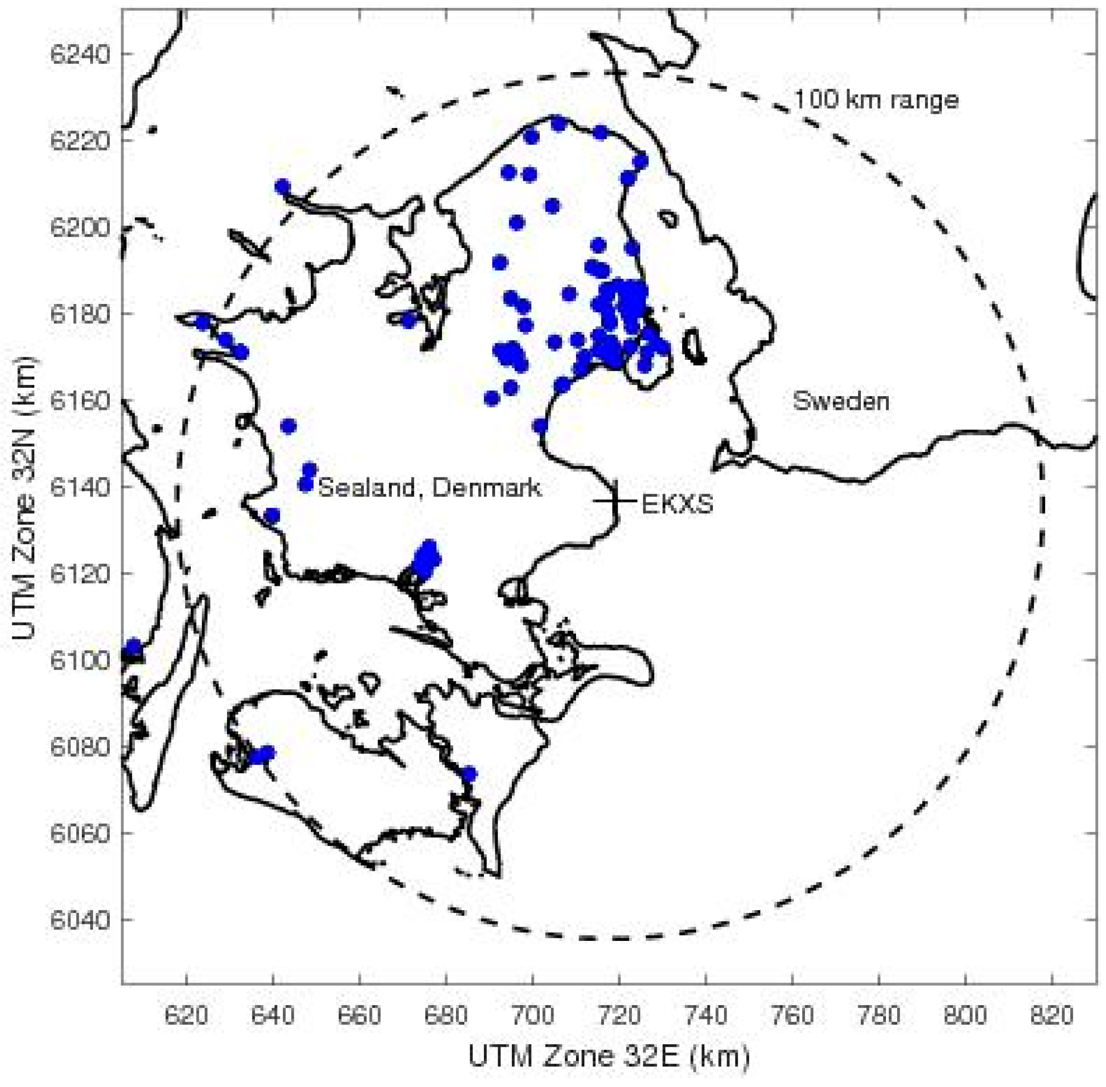
Details of radar rainfall data presented in this paper are described in Thorndahl et al. [29] covering a period from 2002 to 2012. The dataset is expanded with an additional 4 years to cover the period from 2002 to 2016. The raw radar data is measured with a single C-band Doppler radar (manufactured by EEC, Enterprise, AL, USA) and operated by the Danish Meteorological Institute (DMI). The total range of the radar is 240 km, and the 100 km range will be used for quantitative precipitation estimates. This range covers an area of ~31,400 km2, including the greater Copenhagen area and the island of Sealand in Denmark as well as parts of south-western Sweden (Figure 1). The spatial resolution of the cartesian rainfall product is 500 × 500 m2 generated in a 1 km altitude pseudo-CAPPI layer. This product is selected due to consistency in data having a fixed elevation as a function of range and significantly fewer errors and clutter compared to lower altitude pseudo CAPPI products. The temporal resolution of the original dataset is 10 min, but the developed dataset has been regenerated by using a mixed forward and backward advection interpolation method by Nielsen et al. [30] to a 1 min resolution. Radar reflectivity is converted into rainfall intensities using a fixed Marshall–Palmer relationship [31] and bias-adjusted against with 67 rain stations/gauges using a daily mean field bias adjustment approach as described in Thorndahl et al. [30] and Smith and Krajewski [32]. As documented in Thorndahl et al. [29], the mean-field bias adjustment is applied within the 100 km range domain of the radar on a daily time scale. Regional variability of the bias is insignificant and can be neglected [29].
The rain gauge/radar pairs applied to calculate the daily bias consists of only one rain station/gauge per 500 × 500 m2 pixel. For this study, 534 individual rainy days with more than 1 mm of rainfall (in at least one of the rain stations/gauges) were selected. All days with significant noise (defect filters), missing images due to hardware or communication failures, poor bias adjustment (defined as a Nash–Sutcliffe Efficiency below 0, e.g., due to little gauge data, gauge data failures) were omitted. Consequently, the dataset consists of 534 discrete days and is thus discontinuous for the period (2002–2016). In traditional rainfall design statistics of rainfall, an incomplete dataset with periods of missing data is subject to uncertainty in the estimation of return periods. However, since this study disregards estimating return periods, the discontinuous data are not considered any further.
2.2. Correction for Pixel Scale Error
In the rain gauge-based development of ARFs, the areal component is usually estimated by interpolating over a number of rain stations/gauges using a spatial interpolation technique, such as kriging, inverse distance weighting, or Thiessen polygons. With the use of radar data, it is not necessary to interpolate in space. However, there is a need to know the “true” point rainfall. Even with a fairly high spatial resolution of 500 × 500 m2 as applied here, there is a need to acknowledge the scale error between rain gauge and radar pixel [25,33,34,35,36,37]. This representativeness error between rain gauge and radar can originate from several sources. It can be due to rainfall variability itself within a radar pixel meaning that the average rainfall over a 500 × 500 m2 is not the same as recorded in a rain gauge with a surface area of less than 0.05 m2. It can also be due to artefacts measuring with radars, such as the difference between the atmosphere and ground, wind drift, timing errors. Rather than attempting to estimate the rainfall variability at subpixel scale, a data-driven approach for estimation of the mean error is suggested in this paper. This involves calculating a ratio between maximum intensities at different durations (aggregation levels) from rain gauge and radar, respectively. The estimation of the pixel scale error is thus represented through duration-dependent bias factor
where iG is the rainfall intensity from rain stations/gauges (G) averaged over the duration d, and correspondingly iR is the rainfall intensity averaged over duration d which is calculated from daily mean-field bias adjusted radar (R) estimates based on Thorndahl et al. [29]. n is the total number of rain station/gauge radar pixel pairs within the radar range for a specific day t. T is the total number of selected rainy days. The max function implies that the maximum the daily maximum intensity over duration d is applied in rain gauge data and radar, respectively. The developed biases are presented in the result section.
2.3. Method Development
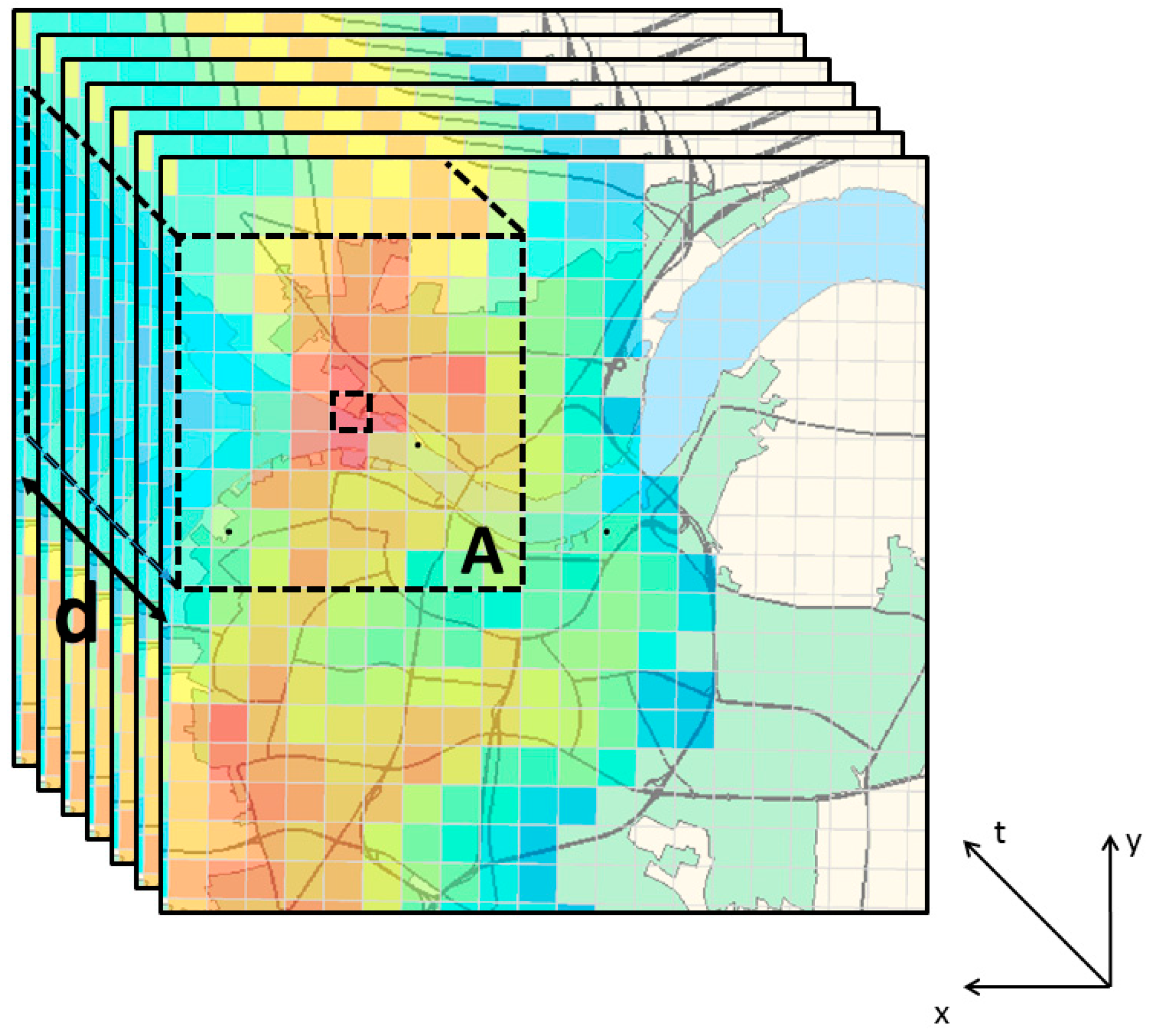
Radar rainfall data from the database are averaged in time and space applying N-dimensional convolution in MATLAB using discrete values of rainfall duration d and area A. A principle sketch of the averaging procedure is shown in Figure 2.
The areal reduction factor (ARF) is defined by the ratio between the maximum radar rainfall intensity (iR,max), averaged over duration d, area A and the maximum rainfall intensity in a point (A→0). Since a storm-centred approach is applied, the maximum point rainfall, is estimated in the point of the maximum rain intensity within the extent of the averaged area, A, (Figure 2). For each rainy day and selected discrete values of A and d, the maximum radar rainfall intensity within the domain iR,max is calculated. In this paper, the combination of rainy day, A and d defines a storm, s. The estimation of the ARF is conducted for a number of individual storms (s).
The storm definition allows for multiple locations (within the domain) of the paired areal and point maximum rainfall intensity, depending on duration and area within the same rainy day. It is a key feature of the storm-centred approach that the location is not fixed. A limit of the storm definition is that only one peak (maximum intensity and location of maximum intensity) per storm can be selected.
The ratio of the maximum areal intensity for a given duration with the maximum point intensity over the same duration is calculated. As presented in the data section, the “true” point rainfall is unknown. Instead of the point rainfall, the average rainfall over a pixel size, p is applied. The derived bias Equation (1) between rain station/gauge and radar a function of duration is applied to account for the pixel scale error. The ARF can thus be estimated by
To approximate the individual ARF relationships to a more generic relationship of the ARF as a function of duration and area, recognised methods from the literature are employed in the next sections. Following Rodriguez-Iturbe and Mejía [4] and Sivapalan and Blöschl [5], the ARF is assumed to be exponentially dependent on the ratio between the distance between two points and the correlation length, λ.
where λ is the correlation length and is defined as the scaled area.
Other authors (e.g., Villarini et al. [38]) have expanded this relationship to allow for the ARF to depend on arbitrary parameters:
where c1 and c2 are coefficients calibrated from record data. Based on the ARF as a function of area, λ is calibrated for each duration and storm using a non-linear least squares approximation. To limit the degrees of freedom, Equation (4) (i.e., Equation (5) with parameters c1 = 0.5 and c2 = 0.5) is initially applied to fit the ARF.
The novelty of this study is to develop a relationship between λ and d. Preliminary analysis of record values of λ for each duration suggests using a power-function approximation described by the following equation:
Implementing this expression in Equation (5) leads to the following relationship:
Applying the relationship developed in Equation (6), the parameters c1 and c2 (Equation (5)) are fitted by the non-linear least squares approximation method. This leads to a modification of the initial values of parameters from Equation (4). In this way, all four parameters are calibrated, and Equation (7) can be simplified to the following relationship:
where , , and .
Thus, Equation (8) is developed as a 3-parameter relationship of the ARF as a function of area and duration. The parameters b1, b2, and b3 will be calibrated by a stepwise procedure of Equations (3), (4), (6–8). The calibration procedure is explained along with the data-processing and examples in the results section.
3. Application and Results
The analyses conducted in this paper apply discrete values of durations and areas. The averaging of radar data in space and time is quite computationally demanding, and it is, therefore, not feasible to apply finer intervals. The following values of durations are applied: 1, 10, 30, 60, 90, 180, 240, 360, 540, 720, 1080, and 1440 min along with 20 intervals of the area ranging from 0.25 km2 (one pixel) to 100 km2 (20 × 20 pixels). This corresponds to 240 combinations of area and duration for each of the 534 storms leading to 6408 individual storm-centred areal reduction factor relationships.
Development procedure:
- (1)
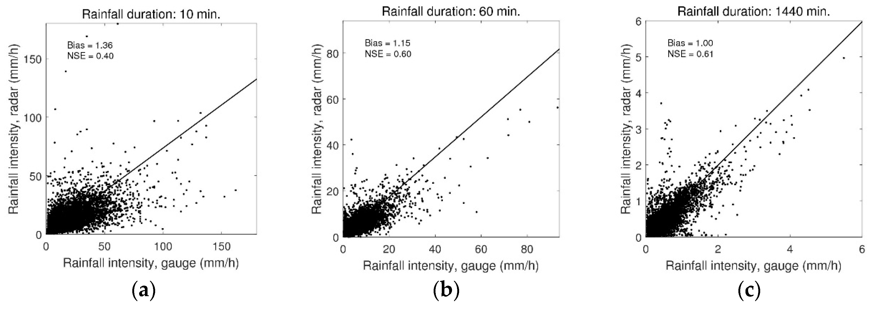
- Applying Equation (1), a correction of the pixel scale error is performed. Results are shown for selected durations in Figure 3 and Table 1. It is evident that the error between rain gauge intensities and radar intensities are significantly larger for short rainfall durations. This is a result of the daily mean-field bias adjustment and leads to a bias factor of 1 for the 1440 min durations (1 day). As shown in Figure 3, there is a considerable scatter between maximum rain gauge intensities and the corresponding radar intensities, which is also explained by the Nash–Sutcliffe Efficiency (NSE)-values in Table 1 and Figure 3. Furthermore, the scatter is larger for the shorter durations indicating high uncertainties. However, as the study aims for a mean pixel scale error, the dispersion of the pixel scale error is not considered any further.
- (2)
- (3)
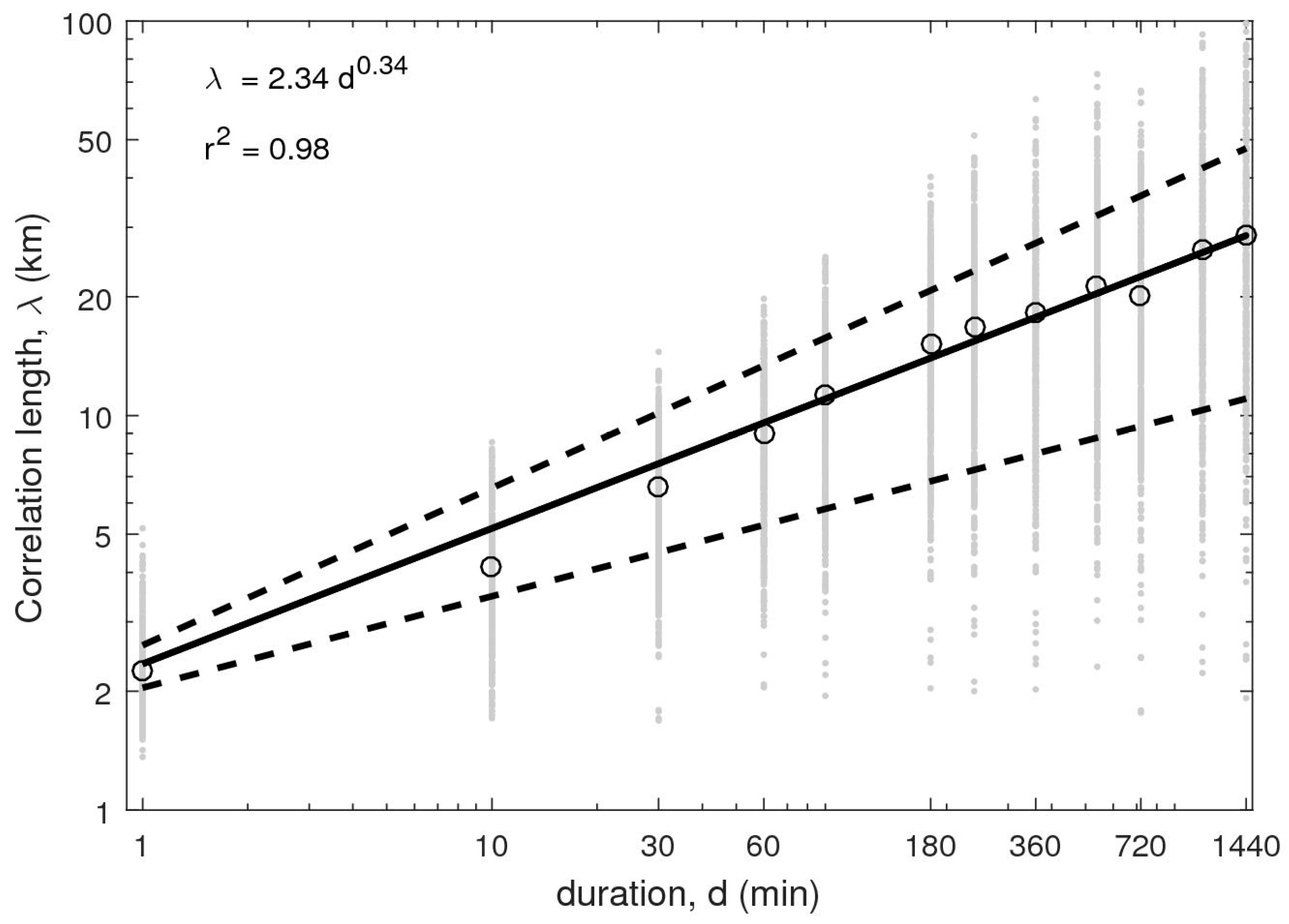
- The correlation lengths, λ are fitted (Equation (6)) as a function of duration (Figure 6). From Figure 6, it is evident that there is a large variability from storm to storm, but that the mean fit well to the power function with r2 of 0.98. It shows that the power-law function in Equation (6) can be further used to derive a relationship of the storm-centred ARF as a function of area and duration. In addition to the mean relationship, the uncertainty corresponding to mean plus/minus one standard deviation (assuming a Gaussian distribution) is investigated. This uncertainty will provide insight into the variability from storm to storm.
- (4)
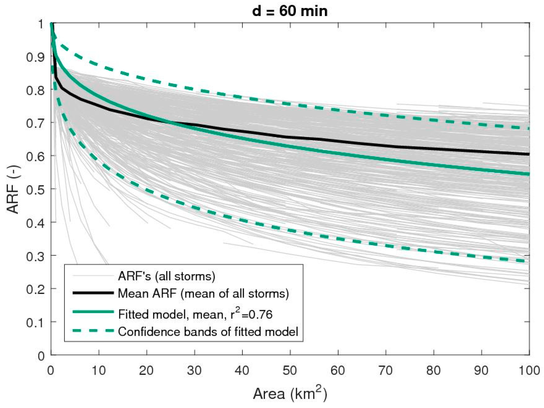
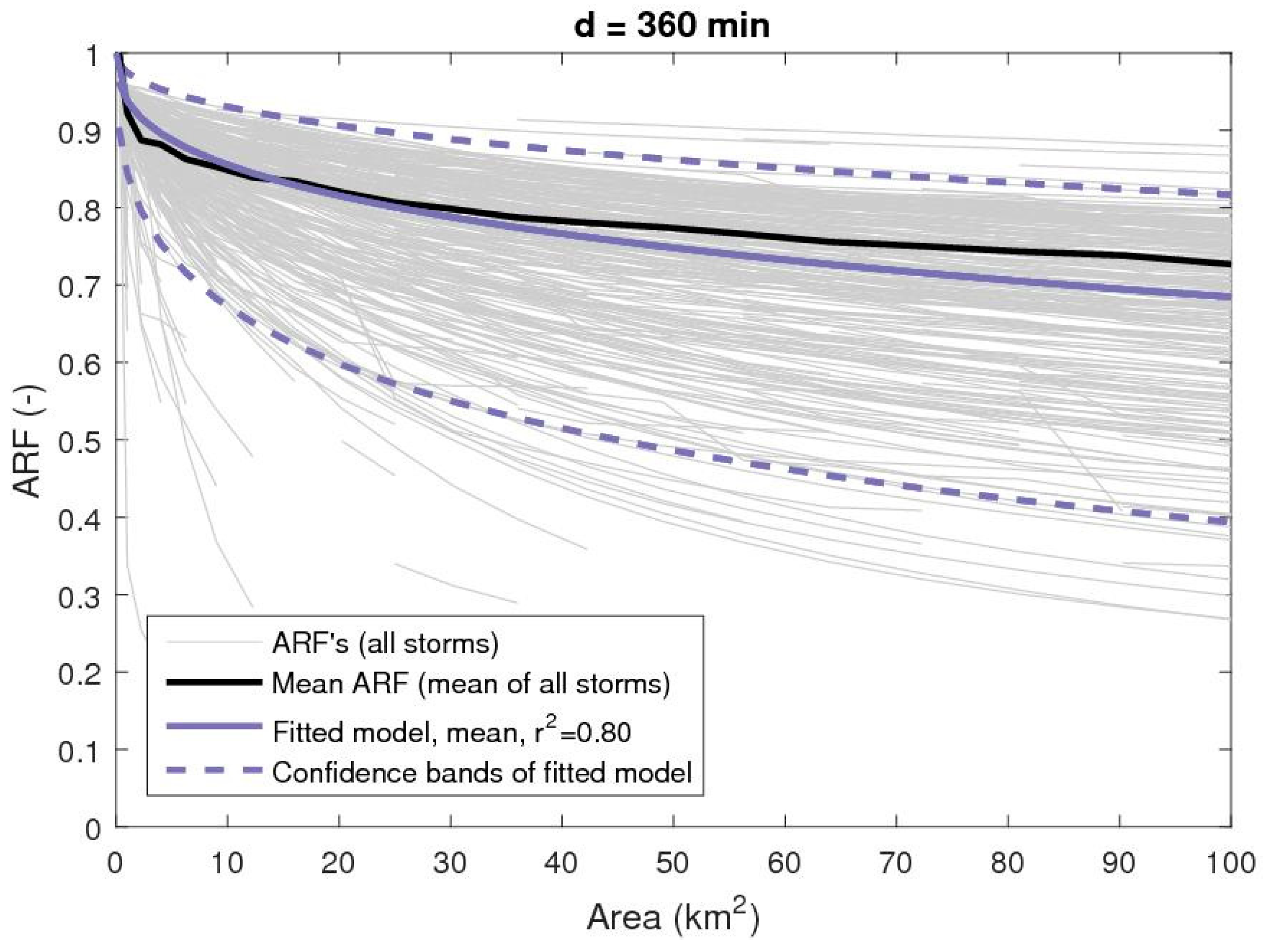
- Applying the obtained function of correlation length and duration, each storm is re-fitted by the relationship in Equation (7) to derive an ARF function. Examples of this fit are shown in Figure 4 and Figure 5 for durations of 60 and 360 min, respectively. Comparing with the mean ARF functions, the fitted relationships show a slight overestimation for the small areas and correspondingly an underestimation for large areas. For some durations, the opposite case occurs (not shown). This uncertainty is a trade-off of fitting a fixed parameter relationship to all durations.
- (5)
It is evident that the variability from storm to storm of the storm-centred ARF functions is large compared to mean and fitted ARF curves in Figure 4 and Figure 5. This large variability of the storm-centred approach is also shown by Wright et al. [18] for an American radar rainfall dataset in North Carolina. The variability indicates that a variety of different storms is represented in the dataset, i.e., both short convective thunderstorms with a small spatial extent and more widespread rainfall which occurs during stratiform conditions.
4. Discussion
In order to apply developed ARF relationships in design of urban drainage systems, one approach would be to link the extreme event statistics (design rainfall) to the ARF-relationship, e.g., by introducing an ARF which is also dependent on the average return period of the design rainfall as presented in Lombardo et al. [16] and Overeem et al. [17]. Because a discontinuous and incomplete radar dataset over the observation period of 15 years is used (as presented in the data section), it is not possible to derive the return periods for rainfall intensities. Likewise, it is not possible to directly transfer the ARF relationships to design rainfall. This is a limitation of this study. In comparison with other studies, the rainfall database contains a large quantity of data over a large domain, and a significantly better description of the spatial rainfall variability, than if rain station/gauge records were used alone. This means that the ARF relationships are based on more data than previous studies (see Section 4.1). This enhances the validity of the study.
If average return periods of design rainfall were linked to ARF relationships, it would require the application of an area-fixed approach instead of the storm-centred approach. Due to the reasons indicated above, this is a subject of further investigations. Following the argument of Wright et al. [18], there are also difficulties using the area-fixed approach, in terms of representing the “true” properties of more extreme events (i.e., longer return periods). In their conclusions, this might lead to larger ARF values (compared to the storm-centred approach), thus to overestimation of design rainfall and again to oversizing of urban drainage systems to be designed. Whether the area-fixed approach would result in different ARF relationships are in this case, a subject of further investigation. This study, however, limits to conclude that there is a quantifiable uncertainty of the ARF relationships from storm to storm, which is important to consider in any design phase.
The dependence of the return period is not supported by the findings of Wright et al. [18] who argue that it is an artefact of the chosen method. Furthermore, it is questionable if the maximum point rainfall would have the same return period as the maximum areal rainfall since they might originate from very different weather types (i.e., convective vs. stratiform storms). This is thus an argument in favour of using the storm-centred approach where the maximum areal and maximum point rainfall occur at the same time. Whether or not the return period dependence is present or whether it should be considered in urban drainage design, is thus an open question. Again, this study acknowledges the variability in the ARF from storm to storm and suggests that mean values ARFs plus/minus one or two standard deviations are used according to the required safety in the design.
4.1. Comparison with Previous Studies
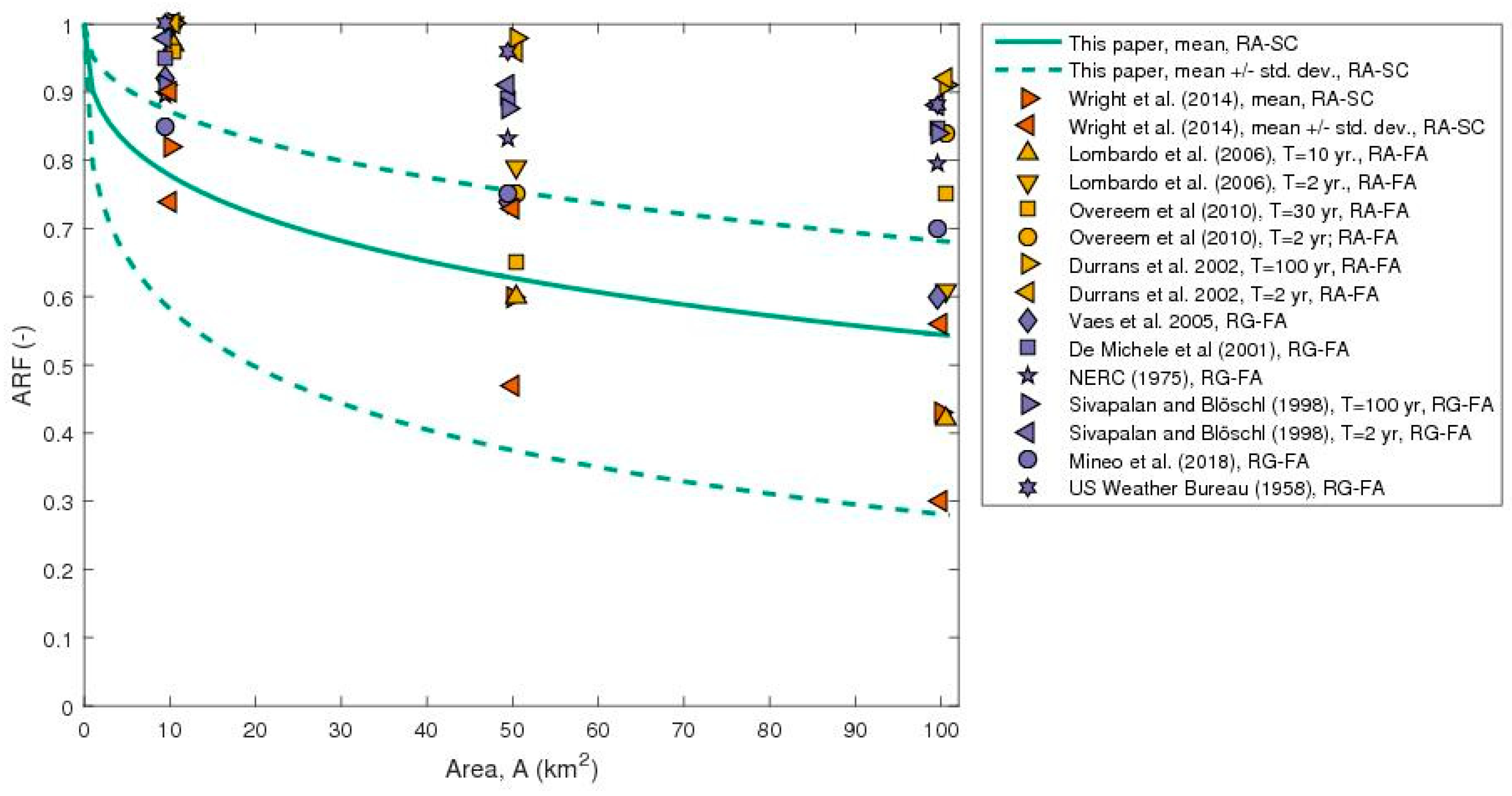
To discuss the generalisation of results, an example of the variability of ARFs found in the previous studies are given below. This highlights how the ARFs vary depending on the method, data quantity and quality, national guidelines or experience, choice of spatial interpolation method (for rain gauge data), location, climate, etc. Values relevant within an urban hydrological context, i.e., ARFs for 1 h durations with areas of 10, 50, and 100 km2 are examined in Figure 8. Few authors [11,16,17,25] have reported ARFs for sub-hourly durations and areas less than 100 km2. This comparison is not exhaustive, but it gives an indication of differences between ARF values using the area-fixed or storm-centred approach as well as differences using rain gauge and radar data.
From Figure 8, there is a tendency for ARFs derived from rain gauge data to show higher values than the radar data counterparts. Furthermore, there is a tendency for storm-centred ARFs derived in this paper and in Wright et al. [18] to be smaller than the ones found using area-fixed approaches. Smaller values of the storm-centred approach in comparison to the area-fixed have also been stated in Sivapalan and Blöschl [5]. Many of the fixed-area ARFs have been developed for much larger spatial scales (e.g., up to 20,000 km2, [15]) and for rainfall durations of 1 day or more. Calibrated relationships which cover these large rural scales might potentially be less precise on smaller scales relevant in urban hydrology. It is acknowledged that the ARFs derived in this paper are smaller than the ones reported in the majority of previous studies. Mean values and standard deviations are, however, comparable to the ones reported by Wright et al. [18], which implies that the storm-centred approach will provide larger areal reductions, thus smaller ARFs, compared to the fixed-area counterparts. From the comparison, it is not possible to determine whether ARFs obtained from rain gauge data is different from the ones based on radar data.
4.2. Implementation in Urban Drainage Design
As stated in the introduction, it has not previously been a part of the code of practice in Denmark to account for the spatial variability of rainfall in the design of urban drainage systems. Thus an ARF equal to 1 has been applied independently of design duration and catchment area. Introduction of the ARF will lead to a reduction in the design rainfall intensities for increasing catchment sizes. Following Allen and DeGaetano [15], Lombardo et al. [16] and Overeem et al. [17], increasing the average return period will also give reason to decrease the ARF and thus, the design rainfall intensity. Relating this to the mean and confidence intervals presented in Figure 4 and Figure 5 will entail that the upper confidence limit (mean + 1 × std. dev.) will correspond to lower return periods, and the lower confidence limit (mean – 1 × std. dev.) will correspond to higher return periods. Since design rainfall intensities will increase as a function of increasing return period, the ARF would counteract and lead to smaller values; thus, smaller design rainfall intensities for increasing return periods. It is therefore argued, that it would be on the safe side to use the mean ARF, but still, a significant reduction of the design rainfall compared to neglecting the areal component. It is recommended that the best option is to use the mean ARF as the most probable value with lower and upper confidence limits of +/− 1 standard deviation.
Whilst most other authors have focused on developing areal reduction factors for large hydrological scales, short durations (<1 h) and small catchments (<10 km2) are of importance in urban hydrology. An example relevant to urban scales is presented in the following, along with an evaluation of the impact of the implementation of an ARF.
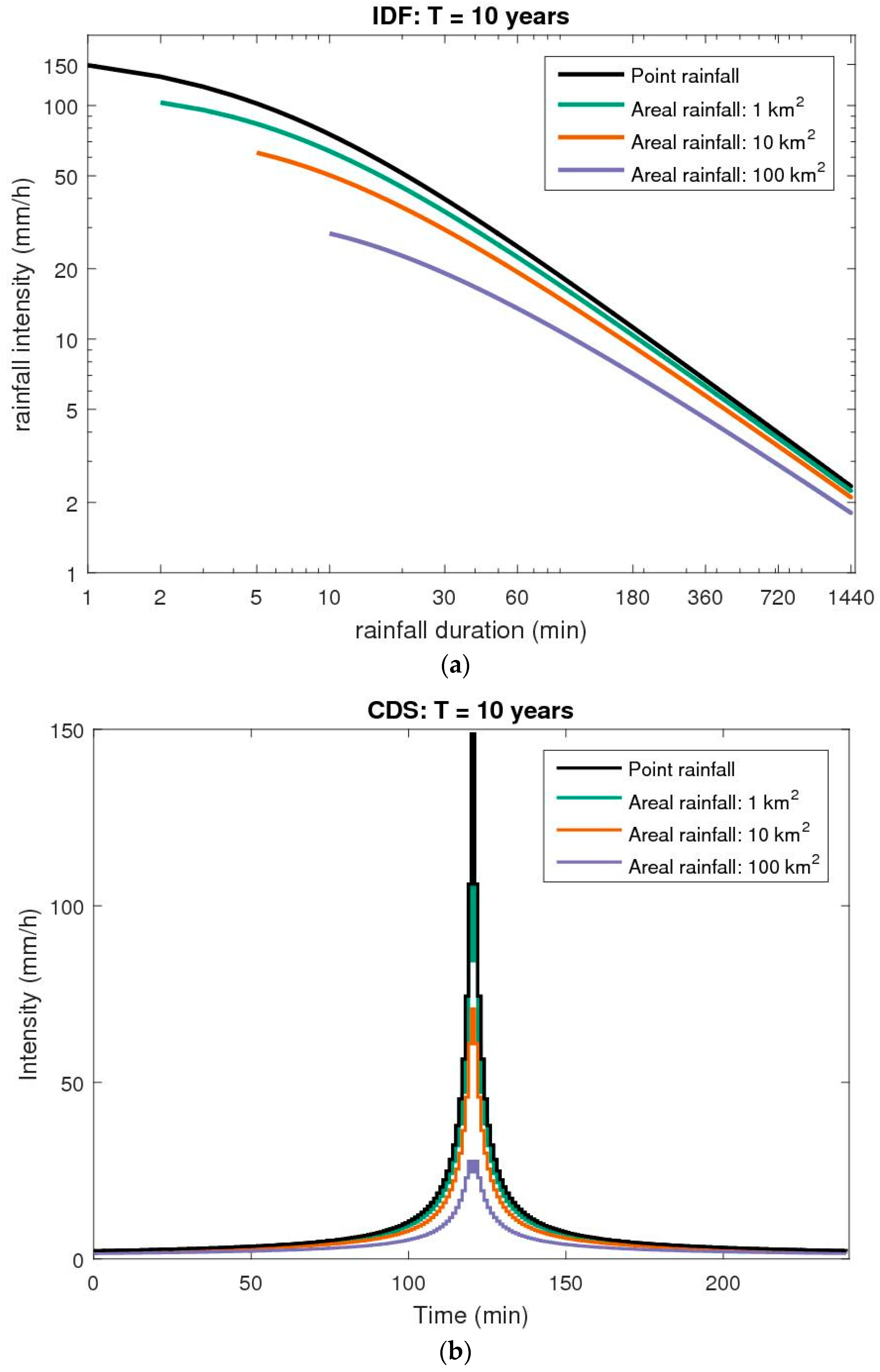
For a catchment of 10 km2 with a time of concentration corresponding to 60 min to the outlet, the developed mean ARF is 0.78 with 0.58 and 0.87 for the lower and upper confidence limits (+/- the standard deviation), respectively. This corresponds to a reduction of the design rainfall on average of 25% ranging from 13% to 46%. Using the mean ARF, the design rainfall for Danish conditions with a return period of 10 years [39] can be adjusted as presented in Figure 9a for IDF curves and Figure 9b for design rainfall of the Chicago design storm (CDS) type [40]. Compared to the current design practice where no areal reduction is implemented; this will reduce the design intensities and thus lead to smaller designs.
5. Conclusions
In this paper, storm-centred areal reduction factor relationships were developed from a radar rainfall dataset covering a period of 15 years. A novel and generic 3-parameter relationship describing the areal reduction factors as a function of rainfall duration and area has been derived and calibrated against 6408 individual combinations of storm, area, and duration. The results showed that there is a large variability in the developed ARFs for individual storms; however, using mean values of the developed ARF, combined with confidence limits, provides a reliable method to adjust rainfall for urban drainage design purposes. Impacts of using the storm- centred approach, compared to the more traditional area-fixed approach linked to average return periods of design rainfall, is however still subject to further investigations.
The derived areal reduction factor relationships highlight the importance of accounting for areal rainfall variability in the design of urban drainage systems with catchments as small as 10 km2 with short concentration times (thus short rainfall design durations), to prevent unnecessary oversizing of designs.
Author Contributions
Conceptualisation, methodology, formal analysis, and writing—original draft preparation, S.T. Software, writing—review and editing, and validation, J.E.N. Project administration writing—review and editing, and validation, M.R.R.
Funding
This research was partially funded by Aarhus Water and VUDP (Vandsektorens Udviklings-og Demonstrations program, Denmark, project ID 1162.2017).
Acknowledgments
The authors would like to thank the Danish Meteorological Institute for the use of radar data and the Danish Wastewater Committee under the Society of Danish Engineers for rain station/gauge data.
Conflicts of Interest
The authors declare no conflict of interest.
References
- Willems, P. Compound intensity/duration/frequency-relationships of extreme precipitation for two seasons and two storm types. J. Hydrol. 2000, 233, 189–205. [Google Scholar] [CrossRef]
- Madsen, H.; Arnbjerg-Nielsen, K.; Mikkelsen, P.S. Update of regional intensity-duration-frequency curves in Denmark: Tendency towards increased storm intensities. Atmos. Res. 2009, 92, 343–349. [Google Scholar] [CrossRef]
- WPC Funktionspraksis for afløbssystemer under regn, skrift nr. 27 (Practice for drainage systems during rain, Guideline no. 27); The Water Pollution Committee of the Society of Danish Engineers; IDA: Copenhagen, Denmark, 2007. [Google Scholar]
- Rodriguez-Iturbe, I.; Mejía, J.M. On the transformation of point rainfall to areal rainfall. Water Resour. Res. 1974, 10, 729–735. [Google Scholar] [CrossRef]
- Sivapalan, M.; Blöschl, G. Transformation of point rainfall to areal rainfall: Intensity-duration-frequency curves. J. Hydrol. 1998, 204, 150–167. [Google Scholar] [CrossRef]
- Villarini, G.; Serinaldi, F.; Krajewski, W.F. Modeling radar-rainfall estimation uncertainties using parametric and non-parametric approaches. Adv. Water Resour. 2008, 31, 1674–1686. [Google Scholar] [CrossRef]
- U.S. Weather Bureau. Rainfall Intensity-Frequency Regime Part 2-Southeastern United States, Technical Paper No. 29; Department of Commerce: Washington, DC, USA, 1958.
- NERC (Natural Environment Research Council, UK). Flood Studies Report; Natural Environment Research Council: Swindon, UK, 1975; Volume II. [Google Scholar]
- Asquith, W.H.; Famiglietti, J.S. Precipitation areal-reduction factor estimation using an annual-maxima centered approach. J. Hydrol. 2000, 230, 55–69. [Google Scholar] [CrossRef] [Green Version]
- De Michele, C.; Kottegoda, N.T.; Rosso, R. The derivation of areal reduction factor of storm rainfall from its scaling properties. Water Resour. Res. 2001, 37, 3247–3252. [Google Scholar] [CrossRef]
- Vaes, G.; Willems, P.; Berlamont, J. Areal rainfall correction coefficients for small urban catchments. Atmos. Res. 2005, 77, 48–59. [Google Scholar] [CrossRef]
- Veneziano, D.; Langousis, A. The areal reduction factor: A multifractal analysis. Water Resour. Res. 2005, 41, 1–15. [Google Scholar] [CrossRef]
- Mineo, C.; Ridolfi, E.; Napolitano, F.; Russo, F. The areal reduction factor: A new analytical expression for the Lazio Region in central Italy. J. Hydrol. 2018, 560, 471–479. [Google Scholar] [CrossRef]
- Durrans, S.R.; Julian, L.T.; Yekta, M. Estimation of Depth-Area Relationships using Radar-Rainfall Data. J. Hydrol. Eng. 2007, 7, 356–367. [Google Scholar] [CrossRef]
- Allen, R.J.; DeGaetano, A.T. Considerations for the use of radar-derived precipitation estimates in determining return intervals for extreme areal precipitation amounts. J. Hydrol. 2005, 315, 203–219. [Google Scholar] [CrossRef]
- Lombardo, F.; Napolitano, F.; Russo, F. On the use of radar reflectivity for estimation of the areal reduction factor. Nat. Hazards Earth Syst. Sci. 2006, 6, 377–386. [Google Scholar] [CrossRef] [Green Version]
- Overeem, A.; Buishand, T.A.; Holleman, I.; Uijlenhoet, R. Extreme value modeling of areal rainfall from weather radar. Water Resour. Res. 2010, 46, 1–10. [Google Scholar] [CrossRef]
- Wright, D.B.; Smith, J.A.; Baeck, M.L. Critical Examination of Area Reduction Factors. J. Hydrol. Eng. 2014, 19, 769–776. [Google Scholar] [CrossRef]
- Pavlovic, S.; Perica, S.; St Laurent, M.; Mejía, A. Intercomparison of selected fixed-area areal reduction factor methods. J. Hydrol. 2016, 537, 419–430. [Google Scholar] [CrossRef]
- Svensson, C.; Jones, D.A. Review of methods for deriving areal reduction factors. J. Flood Risk Manag. 2010, 3, 232–245. [Google Scholar] [CrossRef] [Green Version]
- Omolayo, A.S. On the transposition of areal reduction factors for rainfall frequency estimation. J. Hydrol. 1993, 145, 191–205. [Google Scholar] [CrossRef]
- Schilling, W. Rainfall data for urban hydrology: what do we need? Atmos. Res. 1991, 27, 5–21. [Google Scholar] [CrossRef]
- Einfalt, T.; Arnbjerg-Nielsen, K.; Golz, C.; Jensen, N.-E.; Quirmbach, M.; Vaes, G.; Vieux, B. Towards a roadmap for use of radar rainfall data in urban drainage. J. Hydrol. 2004, 299, 186–202. [Google Scholar] [CrossRef]
- Thorndahl, S.; Einfalt, T.; Willems, P.; Nielsen, J.E.; ten Veldhuis, M.-C.; Arnbjerg-Nielsen, K.; Rasmussen, M.R.; Molnar, P. Weather radar rainfall data in urban hydrology. Hydrol. Earth Syst. Sci. 2017, 21, 1359–1380. [Google Scholar] [CrossRef] [Green Version]
- Bengtsson, L.; Niemczynowicz, J. Areal reduction factors from rain movement. Nord. Hydrol. 1986, 17, 65–82. [Google Scholar] [CrossRef]
- Thorndahl, S.; Beven, K.J.; Jensen, J.B.; Schaarup-Jensen, K. Event based uncertainty assessment in urban drainage modelling, applying the GLUE methodology. J. Hydrol. 2008, 357, 421–437. [Google Scholar] [CrossRef] [Green Version]
- Thorndahl, S.; Willems, P. Probabilistic modelling of overflow, surcharge and flooding in urban drainage using the first-order reliability method and parameterization of local rain series. Water Res. 2008, 42, 455–466. [Google Scholar] [CrossRef]
- Thorndahl, S.; Schaarup-Jensen, K.; Rasmussen, M.R. On hydraulic and pollution effects of converting combined sewer catchments to separate sewer catchments. Urban Water J. 2013, 12, 120–130. [Google Scholar] [CrossRef]
- Thorndahl, S.; Nielsen, J.E.; Rasmussen, M.R. Bias adjustment and advection interpolation of long-term high resolution radar rainfall series. J. Hydrol. 2014, 508, 214–226. [Google Scholar] [CrossRef]
- Nielsen, J.E.; Thorndahl, S.; Rasmussen, M.R. A numerical method to generate high temporal resolution precipitation time series by combining weather radar measurements with a nowcast model. Atmos. Res. 2014, 138, 1–12. [Google Scholar] [CrossRef]
- Marshall, J.S.; Palmer, W.M. The distribution of raindrops with size. J. Meteor 1945, 5, 165–166. [Google Scholar] [CrossRef]
- Smith, J.A.; Krajewski, W.F. Estimation of the Mean Field Bias of Radar Rainfall Estimates. J. Appl. Meteorol. 2002, 30, 397–412. [Google Scholar] [CrossRef]
- Kitchen, M.; Blackall, R.M. Representativeness errors in comparisons between radar and gauge measurements of rainfall. J. Hydrol. 1992, 134, 13–33. [Google Scholar] [CrossRef]
- Habib, E.; Ciach, G.J.; Krajewski, W.F. A method for filtering out raingauge representativeness errors from the verification distributions of radar and raingauge rainfall. Adv. Water Resour. 2004, 27, 967–980. [Google Scholar] [CrossRef]
- Krajewski, W.F.; Villarini, G.; Smith, J.A. Radar-Rainfall Uncertainties: Where are We after Thirty Years of Effort? Bull. Am. Meteorol. Soc. 2010, 91, 87–94. [Google Scholar] [CrossRef]
- Peleg, N.; Ben-Asher, M.; Morin, E. Radar subpixel-scale rainfall variability and uncertainty: Lessons learned from observations of a dense rain-gauge network. Hydrol. Earth Syst. Sci. 2013, 17, 2195–2208. [Google Scholar] [CrossRef]
- Peleg, N.; Marra, F.; Fatichi, S.; Paschalis, A.; Molnar, P.; Burlando, P. Spatial variability of extreme rainfall at radar subpixel scale. J. Hydrol. 2018, 556, 922–933. [Google Scholar] [CrossRef] [Green Version]
- Villarini, G.; Mandapaka, P.V.; Krajewski, W.F.; Moore, R.J. Rainfall and sampling uncertainties: A rain gauge perspective. J. Geophys. Res. Atmos. 2008, 113, 1–12. [Google Scholar] [CrossRef]
- Madsen, H.; Gregersen, I.B.; Rosbjerg, D.; Arnbjerg-Nielsen, K. Regional frequency analysis of short duration rainfall extremes using gridded daily rainfall data as co-variate. Water Sci. Technol. 2017, 75, 1971–1981. [Google Scholar] [CrossRef] [PubMed]
- Keifer, C.J.; Chu, H.H. Synthetic Storm Pattern for Drainage Design. J. Hydraul. Div. 1957, 83, 1–25. [Google Scholar]
Figure 1.
Domain of radar (EKXS) rainfall dataset and rainfall stations/gauges (blue dots) used of bias adjustment of radar data.
Figure 1.
Domain of radar (EKXS) rainfall dataset and rainfall stations/gauges (blue dots) used of bias adjustment of radar data.

Figure 2.
Principle of averaging radar images spatially over an area (A) and temporally over a duration (d).
Figure 2.
Principle of averaging radar images spatially over an area (A) and temporally over a duration (d).

Figure 3.
Example of estimation of bias between radar and rain gauge intensities at rainfall durations of 10 (a), 60 (b) and 1440 (c) min for the 500 × 500 m2 resolution.
Figure 3.
Example of estimation of bias between radar and rain gauge intensities at rainfall durations of 10 (a), 60 (b) and 1440 (c) min for the 500 × 500 m2 resolution.

Figure 4.
Areal reduction factors (ARF) for durations of 60 min. Dashed lines are the confidence limits (mean +/− std. dev.) of the fitted ARF.
Figure 4.
Areal reduction factors (ARF) for durations of 60 min. Dashed lines are the confidence limits (mean +/− std. dev.) of the fitted ARF.

Figure 5.
ARF for durations of 360 min. Dashed lines are the confidence limits (mean +/− std. dev.) of the fitted ARF.
Figure 5.
ARF for durations of 360 min. Dashed lines are the confidence limits (mean +/− std. dev.) of the fitted ARF.

Figure 6.
Fitted power-function (Equation (6)) between correlation length and rainfall duration in solid black with confidence limits (mean +/− std. dev.) in dashed lines. Grey dots indicate values for individual storms, and black circles indicate mean values for each duration.
Figure 6.
Fitted power-function (Equation (6)) between correlation length and rainfall duration in solid black with confidence limits (mean +/− std. dev.) in dashed lines. Grey dots indicate values for individual storms, and black circles indicate mean values for each duration.

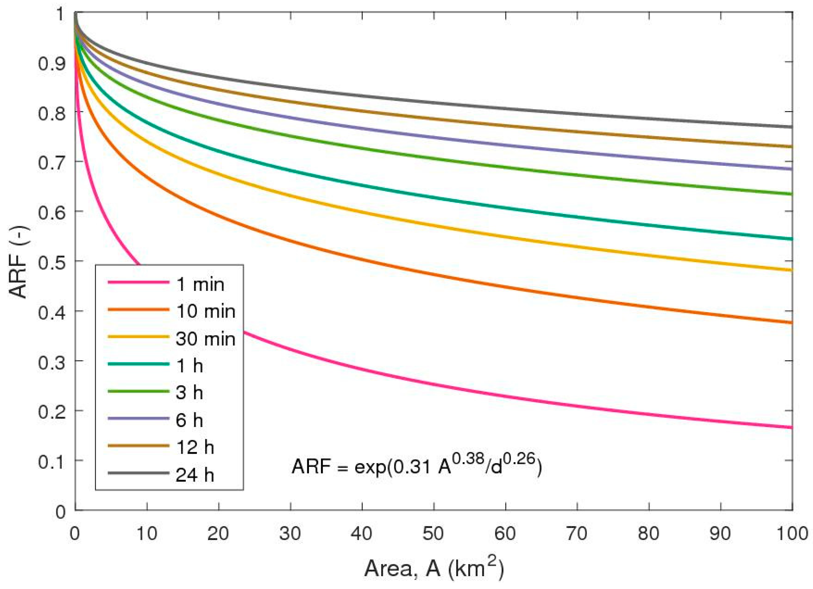
Figure 7.
Mean areal reduction factors as a function of area and duration.

Figure 8.
Derived ARF relationship for 60 min durations compared to previous studies for areas of 10, 50 and 100 km2 estimated using fixed-area (FA) and storm-centred (SC) approaches applying both rain gauge (RG) and radar data (RA).
Figure 8.
Derived ARF relationship for 60 min durations compared to previous studies for areas of 10, 50 and 100 km2 estimated using fixed-area (FA) and storm-centred (SC) approaches applying both rain gauge (RG) and radar data (RA).

Figure 9.
Example of intensity–duration–frequency curves (a) and Chicago design storms (b) with a return period of 10 years [2] adjusted with the developed mean areal reduction factors.
Figure 9.
Example of intensity–duration–frequency curves (a) and Chicago design storms (b) with a return period of 10 years [2] adjusted with the developed mean areal reduction factors.


Table 1.
Bias between radar and rain gauge intensities at different rainfall durations for the pixel size of 500 × 500 m2.
Table 1.
Bias between radar and rain gauge intensities at different rainfall durations for the pixel size of 500 × 500 m2.
| Duration, d (min) | 1 | 10 | 30 | 60 | 180 | 360 | 720 | 1440 |
| Bias, B (-) | 1.63 | 1.36 | 1.21 | 1.15 | 1.07 | 1.04 | 1.03 | 1.00 |
| Nash–Sutcliffe Efficiency, NSE (-) | 0.21 | 0.40 | 0.52 | 0.60 | 0.63 | 0.62 | 0.62 | 0.61 |
| Root mean square error, RMSE (mm/h) | 22.47 | 9.82 | 4.61 | 2.65 | 1.12 | 0.66 | 0.38 | 0.21 |
Table 2.
Calibrated values of the three parameters of Equation (8) for mean and mean +/− std. dev.
| b1 | b2 | b3 | |
|---|---|---|---|
| mean | 0.31 | 0.38 | 0.26 |
| mean – 1 × std. dev. | 0.21 | 0.45 | 0.36 |
| mean + 1 × std. dev. | 0.47 | 0.37 | 0.17 |
© 2019 by the authors. Licensee MDPI, Basel, Switzerland. This article is an open access article distributed under the terms and conditions of the Creative Commons Attribution (CC BY) license (http://creativecommons.org/licenses/by/4.0/).
Share and Cite
MDPI and ACS Style
Thorndahl, S.; Nielsen, J.E.; Rasmussen, M.R. Estimation of Storm-Centred Areal Reduction Factors from Radar Rainfall for Design in Urban Hydrology. Water 2019, 11, 1120. https://doi.org/10.3390/w11061120
AMA Style
Thorndahl S, Nielsen JE, Rasmussen MR. Estimation of Storm-Centred Areal Reduction Factors from Radar Rainfall for Design in Urban Hydrology. Water. 2019; 11(6):1120. https://doi.org/10.3390/w11061120
Chicago/Turabian StyleThorndahl, Søren, Jesper Ellerbæk Nielsen, and Michael R. Rasmussen. 2019. "Estimation of Storm-Centred Areal Reduction Factors from Radar Rainfall for Design in Urban Hydrology" Water 11, no. 6: 1120. https://doi.org/10.3390/w11061120
Note that from the first issue of 2016, this journal uses article numbers instead of page numbers. See further details here.