Runoff Prediction Method Based on Adaptive Elman Neural Network

Abstract

The prediction of medium- and long-term runoff is of great significance to the comprehensive utilization of water resources. Building an adaptive data-driven runoff prediction model by automatic identification of multivariate time series change in runoff forecasting and identifying its influence degree is an attractive and intricate task. At present, the commonly used screening factor method is correlational analysis; others offer multi-collinearity. If these factors are directly input into the model, the parameters of the model tend to increase, and the excessive redundancy and noise adversely affects the prediction results of the model. On the basis of previous studies on medium- and long-term runoff prediction methods, this paper proposes an Elman Neural Network (ENN) adaptive runoff prediction method based on normalized mutual information (NMI) and kernel principal component analysis (KPCA). In this method, the features of the screening factors are extracted automatically by using the mutual information automatic screening factor, and then input into the Elman Neural Network for training. With less features, the parameters of the Elman Neural Network model can be reduced, and the problem of overfitting of the Elman Neural Network model is effectively alleviated. The method is evaluated by using the annual average runoff data of Jinping hydropower station in Chengdu, China, from 2007 to 2011. The maximum relative error of multiple forecasts was found to be less than 16%, and forecast effect was good. The accuracy of prediction is further improved by averaging the results of multiple forecasts.

1. Introduction

Runoff forecasting, especially medium- and long-term runoff forecasting, plays an important role in the comprehensive development, utilization, scientific management and optimization of water resources [1,2,3,4]. Extreme floods, which seem to occur more frequently in recent years (due to climate change), cause immense human suffering and result in enormous economic losses every year worldwide. Therefore, it is necessary to accurately predict the time and size of peak flow before a flood event [5]. Accurate prediction of medium- and long-term runoff is an important prerequisite for guiding the comprehensive development and utilization of water resources, scientific management, and optimal dispatch. Over the past decades, massive runoff forecasting methods and application studies have been carried out at home and abroad. In terms of methods, they can be roughly divided as: data driven model and process driven model. A data-driven model refers to the optimal mathematical relationship between a forecast object (such as annual average runoff) and a predictor (such as the circulation index) based on historical data, regardless of the physical mechanism of the hydrological process. These mathematical relationships can be used to predict future hydrological variables [6]. Traditional methods used to establish mathematical relations include linear regression, stepwise regression [7], local regression, artificial neural networks [8,9,10], and support vector machines [11,12,13]. Meanwhile, a process-driven model requires a hydrological model that can reflect the characteristics of runoff, and future medium- and long-term rainfall information is used as model input to obtain changes in the forecast object [14]. The ensemble streamflow prediction (ESP) method proposed by American scholar Day [15] is a process-driven model and researchers have used this method to study medium- and long-term runoff forecasting in many watersheds. As the mechanism of hydrological process has not been fully elucidated, the applicability of this model is limited [16,17,18,19,20]. Therefore, a data-driven model, especially the runoff prediction model based on neural networks, has become a focused topic for [21,22,23,24] the application of back propagation (BP) neural networks to medium- and long-term hydrological forecasting [25]. In [26,27,28], the application of wavelet neural networks to runoff forecasting was investigated. In [29], the application of gray self-memory based on a BP network model to runoff forecasting was examined. However, these neural network models have two drawbacks: easy fall into local minima and slow convergence [30]. SHAO Yue-hong et al. [31] further evaluate and compare the performance of ENN and land surface hydrological model (TOPX) in the study region.

At present, the commonly used methods for medium and long-term runoff forecasting are based on statistical methods, that is, forecasting is realized by looking for the statistical relationship between the forecasted objects and forecasted factors.

There are three problems in the current statistical methods for medium- and long-term runoff forecasting: First, the hydrological process is complex, and there is a non-linear relationship between the forecasting factors and the forecasting objects, in addition to a linear relationship. Second, principal component analysis (PCA), which is used for noise reduction and redundancy elimination of primary factors, is essentially a linear mapping method, and the principal components obtained are generated by linear mapping. This method ignores the correlation between data higher than the second order, so the extracted principal components are not optimal. Third, the model is used to establish the optimal mathematical relationship between the forecast object and the forecast factor. The commonly used multiple regression is actually a linear fitting, which cannot reflect the nonlinear relationship between the forecast object and the forecast factor. Compared to other models, artificial neural networks for good robustness, strong nonlinear mapping and self-learning ability in long-term runoff forecast has been widely used, but neural network model parameter uncertainty may influence the accuracy of the forecast; there are certain differences in the results with each forecast.

In 1990, Elman proposed the Elman Neural Network and used it to address the voice processing problem [32]. The Elman network is a recurrent neural network with the ability to adapt to time-varying characteristics. Unlike a positive feedback neural network, it has feedback connections originating from the outputs of the hidden layer neurons to its input layer. The state of its neuron depends not only on the current input signal, but also on the previous states of the neuron [33]. Thus, the Elman Neural Network can maintain a sort of state, allowing it to perform tasks such as sequence-prediction [34]. However, relevant research within the domain of medium- and long-term runoff forecasting is very limited.

Compared with previous methods, the main contributions and problems solved in this paper are presented as:

(1) Due to the non-linear relationship of experimental data, we adopted the primary prediction factor method based on NMI, which could not only reflect the nonlinear relationship between variables, but also reflect the nonlinear relationship between variables. NMI overcomes the defect of traditional linear correlation analysis.

(2) KPCA is the nonlinear extension of PCA, that is, the original vector is mapped to the high-dimensional feature space F by mapping function Φ, and PCA analysis is carried out in F. The data in the original space, which are linearly indivisible, are almost linearly separable in the high dimensional feature space. In this instance, PCA is done in a high-dimensional space, and extracted principal components are more represented. Therefore, the feature extraction method based on KPCA greatly improves the processing capacity of nonlinear data and has more advantages than the traditional feature extraction method based on PCA. In addition, the principal components extracted by KPCA are orthogonal to each other, and the data are de-noised and de-redundant, which can well prevent the overfitting of the neural network and improve the generalization ability of the network.

(3) With good robustness, nonlinear mapping, and strong self-learning ability, the artificial neural network can mine the internal relations between the prediction factors and the prediction objects. The Elman neural network selected in this paper is a typical dynamic regression network, which has additional context layers compared with commonly used forward neural networks (such as BP neural network). The context layer can record information from the last network iteration as input to the current iteration, making the Elman network more suitable for prediction of time series data [35]. In addition, the neural network has parameter uncertainty. In order to reduce the uncertainty of prediction, the method of multi-model set prediction is adopted to improve prediction accuracy.

In conclusion, NMI, KPCA and Elman neural network used in this paper have the ability to process non-linear data, except linear data. In addition, the processed data can be de-noised and de-redundant to prevent overfitting of the neural network and improve the generalization ability of the network. The combination of the above three methods overcomes the limitation of traditional methods and improves the stability and accuracy of model prediction. The main purpose of this paper is to build an adaptive data driven runoff forecast [36,37] model, by using the normalized mutual information method to automatically select predictors, and then use the KPCA method to extract features from the selected factors; finally, based on the above, a cyclic neural network model is constructed for runoff prediction. Through the analysis and evaluation of the experimental results, the accuracy of the prediction [38] is improved, and the average annual runoff predicted by a single model. Multiple models are realized based on the Elman neural network, which provides a reference for medium- and long-term runoff prediction [39].

2. Materials and Methods

2.1. Study Area and Data

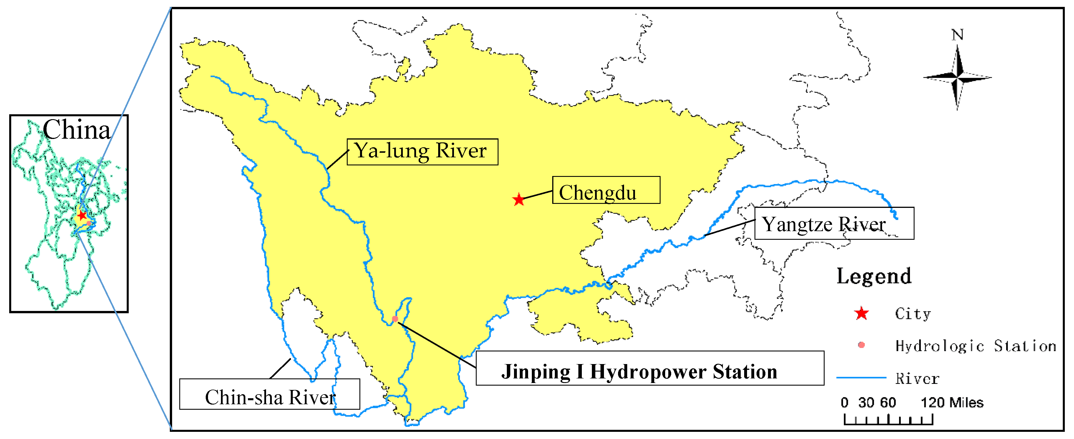
The data source of this study is the Jinping I hydropower station, which is located in the Ya-lung River of Sichuan province, China. The Ya-lung River is the biggest branch of Chin-sha River, which is the upper reaches of the Yangtze River. The reservoir power station is mainly used for power generation, water storage, and flood control. In addition, the drainage area of the reservoir is complex with interlaced mountains and rivers. Therefore, by using the data of this reservoir for research, the experimental data becomes more real and representative. The accurate prediction of runoff in this area is beneficial to the comprehensive development and utilization of water resources in this area, and the experimental model can be simply processed and applied to other areas. The location of Jinping I Hydropower Station is shown in Figure 1. The experimental data in the model used the annual average runoff data of Jinping I Hydropower Station from 1960 to 2011 (provided by the China Institute of Water Resources and Hydropower Research) and the 74 atmospheric circulation parameters from 1959 to 2010 (provided by the National Climate Center of China). Data from 1960–2006 were used to confirm the model, and data from 2007–2011 were used to verify the model.

The average annual flow of the dam site is 1220 m³/s, the average annual flow from June to October in flood season is 2230 m³/s, the average annual flow from November to May in flat and dry season is 493 m³/s, and the average annual runoff is 38.5 billion m³.

2.2. Methodology

The runoff forecasting method presented in this paper consists of three parts: the automatic selection of predictors based on normalized mutual information, the extraction of principal components of predictors based on KPCA, and the forecast of runoff based on a circular neural network. In the following section, these three parts will be elaborated in detail.

2.2.1. Automatic Selection of Predictors for Ranking Mutual Information Correlation

In probability theory and information theory, mutual information is a measure of interdependence between two variables [1]. By calculating the mutual information between the factor time series and the runoff time series, this paper automatically selects the factor that the normalized mutual information is greater than a certain threshold value [40] (usually 0.9), as a predictor according to relevancy. The method of automatically selecting predictors based on mutual information can not only reflect the linear relationship between the factors and runoff, but also the degree of non-linear relationship between them. The traditional method based on linear correlation analysis (Pearson correlation, Spearman correlation) can only respond to the linear relationship between the factors and runoff. Therefore, the factors automatically selected by the correlation ranking method based on mutual information are more representative. The formula for calculating the mutual information between the runoff time series and the factor time series is defined as:

$$MI\left(X,Y\right)={\displaystyle \sum }_{i=1}^n{\displaystyle \sum }_{j=1}^{n}p\left(x_i, y_i\right)\log \left(\frac{p\left(x_i,y_i\right)}{p\left(x_i\right)p\left(y_i\right)}\right) i,j=1,2,3\dots n$$

(1)

where X is the runoff time series, $X={\left(x_1,x_2,x_3\dots x_n\right)}^T$, Y is a factor time series, $Y={\left(y_1,y_2,y_3\dots y_n\right)}^T$, n represents the number of elements in the time series matrix. The molecular $p\left(x_i,y_i\right)$ is a joint distribution law of X and Y, and $p\left(x_i\right)$ and $p\left(y_i\right)$ are the marginal distributions of X and Y, respectively.

For the convenience of comparison, the mutual information needs to be normalized. The value of normalized mutual information is between 0 and 1. The formula for normalized mutual information is:

$$NMI\left(X,Y\right)=2\times \frac{MI\left(X,Y\right)}{H\left(X\right)+H\left(Y\right)}$$

(2)

where $H\left(X\right)$ and $H\left(Y\right)$ are the entropy of X and Y, respectively; $H\left(X\right)$ and $H\left(Y\right)$ are expressed as:

$$H\left(X\right)=-{\displaystyle \sum }_{i=i}^{n}p\left(x_i\right)lo{g}_2\left(p\left(x_i\right)\right)$$

(3)

$$H\left(Y\right)=-{\displaystyle \sum }_{i=i}^{n}p\left(y_i\right)lo{g}_2\left(p\left(y_i\right)\right)$$

(4)

2.2.2. Dimension Reduction of Adaptive Factors of KPCA

KPCA is a nonlinear extension of principal component analysis, which maps the original vector to the high dimensional feature space F through the kernel function $\mathsf{\Phi }$, then carries on the principal component analysis on F. The linear indivisible data in the original space can be linearly separable in the high dimensional feature space, and the principal components extracted in the high-dimensional space are more representative. After PCA transformation, data features can be extracted effectively, which can not only reduce its dimension, but also retain the required recognition information [41]. Therefore, the feature extraction method based on KPCA greatly improves the processing ability of non-linear data, and has more advantages than traditional feature extraction methods based on principal component analysis. In addition, the principal components extracted by the kernel component analysis are orthogonal to each other, and the principal components undergo automatic noise reduction and de-duplication, which can alleviate the cyclic process of neural network overfitting and improve the generalization ability of the network. The process of extracting principal components using KPCA is as follows:

Step 1: Normalize the predictor data selected in the Section 2.2.1 by z-score, as follows:

$$Y^{*}=\frac{Y-\mu }{\sigma }$$

(5)

In the formula, $Y^{*}$ is the normalized data, $Y$ is the predictor data, $\mu$ is the mean value of the time series of $Y$, $\mathsf{\sigma }$ is the standard deviation of $Y$.

Step 2: Calculate the kernel matrix $K$ of the predictor. The calculation formula is obtained as:

$$K=\exp \left(-\frac{\Vert Y_i^{*},Y_j^{*}\Vert {}^2}{2{\sigma }^2}\right)$$

(6)

$Y_i^{*}$ and $Y_j^{*}$, respectively, is a sample of the predictor data $Y^{*}$.

Step 3: Computing the core matrix $K_c$. The calculation formula is:

$$K_c=K-J\times K-K\times J+J\times K\times J$$

(7)

In Equation (7), J is the square matrix of n × n. The specific expression is defined as:

$$J=\left[\begin{array}{ccc}\frac{1}{n}& \dots & \frac{1}{n}\\ ⋮& \ddots & ⋮\\ \frac{1}{n}& \cdots & \frac{1}{n}\end{array}\right]$$

(8)

Step 4: The eigenvalues and eigenvectors of $K_c$ are computed, and the eigenvalues are arranged in order from large to small, and the order of eigenvectors is adjusted according to the eigenvalues.

Step 5: Compute the principal component. The calculation formula is:

$$KPC=K_C{}^{T}A$$

(9)

where A is the normalized eigenvector matrix. A is defined as:

$$A=\left(a_1,a_2,a_i,\cdots ,a_n\right)=\left[\begin{array}{ccc}{a}_{11}& \dots & a_{n1}\\ ⋮& a_i{}_j& ⋮\\ a_{1n}& \cdots & a_{nn}\end{array}\right]$$

(10)

$$\mathrm{where} a_i=\frac{u_i}{\sqrt{{\lambda }_i}},i=1,2,\cdots ,n$$

(11)

${\lambda }_i$ is eigenvalue, and $u_i$ is the eigenvector.

2.2.3. Elman Neural Network Model

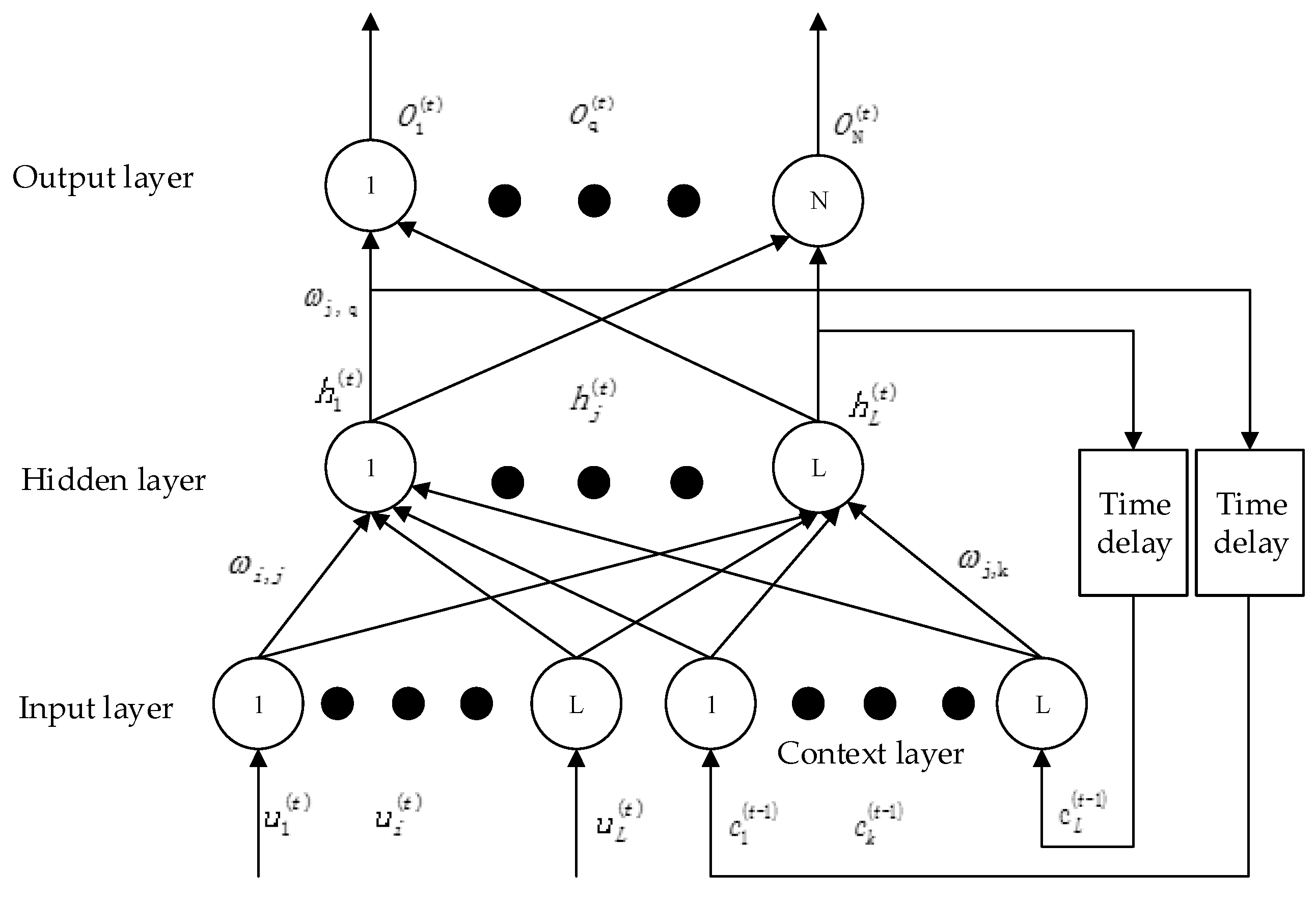
The Elman Neural Network [35], which was first proposed by Elman in 1990 to address the voice processing problem, is a typical dynamic recurrent neural network. The basic configuration of the standard Elman Neural Network consists of an input layer, a hidden layer, an output layer and a context layer. The context layer is a feedback connection from the hidden layer to the input layer. It is worth mentioning that the context layer is able to record information from the last network iteration as input to the current iteration. Therefore, compared with other models, the Elman neural network is more suitable for the prediction of time series data [34]. A standard Elman neural network structure is shown in Figure 2.

The computational process of the Elman network model can be simply expressed as:

The output of the output layer at t time:

$$o_q{}^{\left(t\right)}=f\left({\displaystyle \sum }_{j=1}^L{h}_j{}^{\left(t\right)}{\omega }_{j,q}\right)$$

(12)

The output of the hidden layer at t time:

$$h_j{}^{\left(t\right)}=f\left({\displaystyle \sum }_{i=1}^L{u}_i{}^{\left(t\right)}{\omega }_{i,j}+{\displaystyle \sum }_{k=1}^L{c}_k{}^{\left(t-1\right)}{\omega }_{j,k}\right)$$

(13)

The output of the context layer at t − 1 time:

$$c_k{}^{\left(t-1\right)}=h_j{}^{\left(t\right)}$$

(14)

where the ${\omega }_{j,q}$, ${\omega }_{i,j}$ and ${\omega }_{j,k}$ are the connection weights between the layers, respectively. $f$ is the activation function. In this paper, the activation function of the hidden layer takes the sigmoid function: $f\left(x\right)=\frac{1}{1+e^{-x}}$, and the activation function of the output layer takes the linear function $f\left(x\right)=x$.

The learning process of Elman neural network can be summarized as follows:

Step 1: Use the random function to initialize the connection weights between the layers of the network and determine the allowable error ε for the cost function. Once the network calculates the output of one of the inputs, the cost function calculates the error vector. This error indicates how close our guess is to the expected output. The most commonly used cost functions are the mean square error (MSE), Cross Entropy (CE), and the SVM hinge loss function. Specifically, MSE is better suited to solving the regression problem, which is the prediction of model data. Therefore, in this paper, the mean square error function is used as the cost function, as follows:

$$E=\frac{1}{N}{\displaystyle \sum }_{q=1}^N{\left(O_{eq}^{\left(t\right)}-O_q^{\left(t\right)}\right)}^2$$

(15)

where $O_{eq}^{\left(t\right)}$ is the expected output of the network at t time, $O_q^{\left(t\right)}$ is the actual output of the network (the observed value of the runoff).

Step 2: Normalize the input data, compute the value of E, and update the connection weights between each layer according to E using the momentum gradient descent algorithm. The formula of normalized input data and the formula of weight change are obtained as:

$$z=(z_{\max }-z_{\min })\frac{q-q_{\min }}{q_{\max }-q_{\min }}+q_{\min }$$

(16)

$$\Delta {\omega }^{\left(k\right)}=-\eta \frac{\partial E}{\partial {\omega }^{\left(k\right)}}+\alpha \Delta {\omega }^{\left(k-1\right)}$$

(17)

where $z$ is normalized data, $z_{max}=1,z_{min}=-1,z\in \left(-1,1\right)$, $q$ is the runoff sequence or principal component sequence data, $q_{min}$ is the minimum value in the sequence $q$, $q_{max}$ is the maximum value in the sequence $q$. $\Delta {\omega }^{\left(\mathrm{k}\right)}$ is the change of Elman Neural Network weights in the kth update, $\Delta {\omega }^{\left(\mathrm{k}\right)}$ is the change of Elman Neural Network weights in the k−1th update, $\alpha$ is the momentum constant, $0\le \alpha \le 1$, in this paper, $\alpha =0.9$, $\eta$ is the learning rate, $\eta =0.01$.

Step 3: When the value of E is greater than $\epsilon$, go to step 2 or the end of the study, and compute the output of the network according to Equations (12)–(14).

In addition, in order to stop the Elman Neural Network training process, we set the maximum number of iterative trainings, and when that number is reached, ENN training stops.

2.2.4. Evaluation Criteria

In order to evaluate the performance of the model and the adaptive selection of model structure, the qualified rate (QR), root mean square error (RMSE), mean absolute percent error (MAPE) and mean absolute error (MAE) are adopted as the evaluation criteria. In addition, the reason why we choose QR, RMSE, MAPE and MAE as the evaluation criteria is that these evaluation criteria are sufficient to explain the stability and accuracy of the prediction model.

The formula for the qualified rate is defined as:

$$QR=\frac{m}{n}\times 100\%$$

(18)

where $m$ is the qualified forecast number, $n$ is the total forecast number. If the single forecast error is less than 20%, the forecast is qualified.

The calculation formula of root mean square error can be expressed as:

$$RMSE=\sqrt{\frac{1}{n}{\displaystyle \sum }_{t=1}^n{(q_{sim}^{\left(t\right)}-q_{obs}^{\left(t\right)})}^2}QR=\frac{m}{n}\times 100\%$$

(19)

where $q_{sim}^{\left(t\right)}$ is the predicted value, $q_{obs}^{\left(t\right)}$ is the observed value.

The formula for calculating the mean absolute percent error is expressed as:

$$MAPE=\frac{1}{n}{\displaystyle \sum }_{t=1}^n\frac{\left|q_{sim}^{\left(t\right)}-q_{obs}^{\left(t\right)}\right|}{q_{obs}^{\left(t\right)}}\times 100\%$$

(20)

The formula for calculating the mean absolute error is defined as:

$$MAE=\frac{1}{n}{\displaystyle \sum }_{t=1}^n\left|q_{sim}^{\left(t\right)}-q_{obs}^{\left(t\right)}\right|$$

(21)

The Relative Error (RE) is defined as:

$$RE=\frac{q_{sim}^{\left(t\right)}-q_{obs}^{\left(t\right)}}{q_{obs}^{\left(t\right)}}\times 100\%$$

(22)

3. Results and Discussion

3.1. Implementation of the Forecast Case

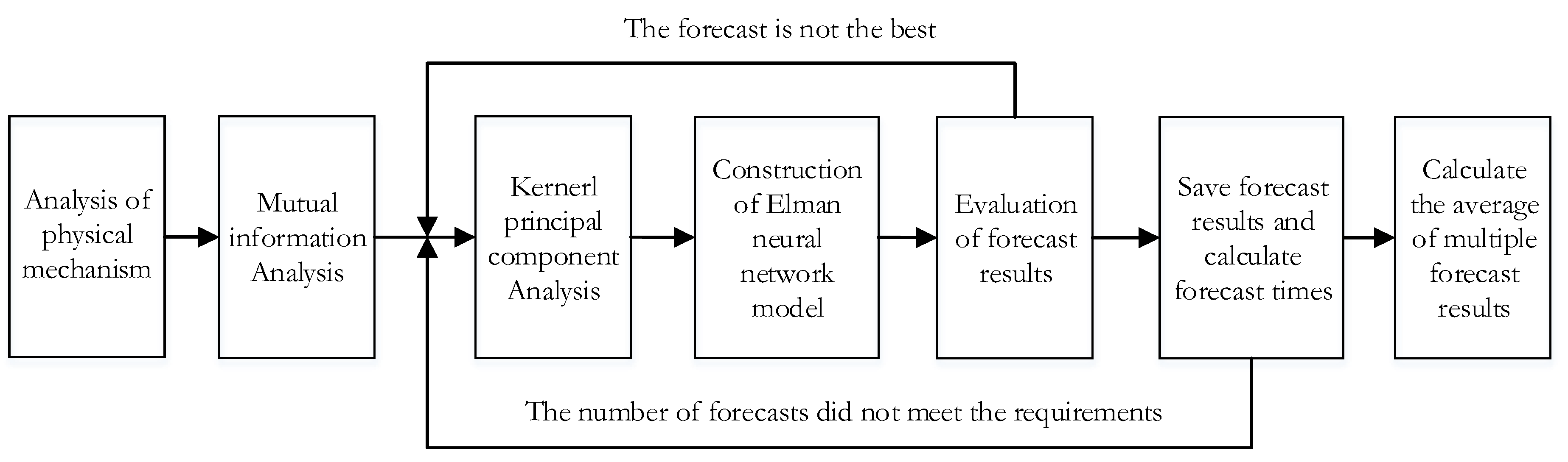
In order to verify its validity, the model proposed in this paper attempts to forecast the annual runoff of Jinping I-Stage hydropower station in Yalong River [42] basin, Sichuan province, China. The detailed automation process is shown in Figure 3.

3.1.1. Determining Forecasting Factor Sets

According to Figure 3, we need to analyze the physical mechanism and use the method of mutual information [43] to filter the predictors:

Step 1: Collect historical runoff data from the research area and meteorological hydrological data that can be used as predictors. Commonly used meteorological hydrological data include atmospheric circulation characteristics, high altitude pressure field, and sea surface temperature index. The data collected in this study include the annual average runoff data of the dam section of Jinping I-Stage hydropower station for 1960–2011 and monthly 74 circulation characteristics data for 1959–2010.

Step 2: Because the forecast object is the average annual runoff, the factor cannot choose from the time of the same year, at the same time considering that the influence of meteorological factors on runoff has hysteresis [44]; thus, a one-by-one correspondence between annual average runoff of Jinping I-Stage hydropower station and 74 atmospheric circulation indices of the previous year was established. The corresponding relationship between the time series of a certain atmospheric circulation index and the runoff time series is shown in

Table 1. The corresponding relationship between the time series of a certain atmospheric circulation index and the runoff time series.

Annual Runoff Time Series	An Exponential Time Series of Atmospheric Circulation
Annual runoff in 1960	Data in January 1959	Data in February 1959	…	Data in December 1959
Annual runoff in 1961	Data in January 1960	Data in February 1960	…	Data in December 1960
Annual runoff in 1962	Data in January 1961	Data in February 1961	…	Data in December 1961
…	…	…	…	…
Annual runoff in 2009	Data in January 2008	Data in February 2008	…	Data in December 2008
Annual runoff in 2010	Data in January 2009	Data in February 2009	…	Data in December 2009
Annual runoff in 2011	Data in January 2010	Data in February 2010	…	Data in December 2010

; the others are similar.

As can be seen from Table 1, the first column of the table shows the annual runoff time series from 1960 to 2011, and the second and final columns of the Table represent the exponential time series of atmospheric circulation, in this part detailed listing of each month.

Step 3: The time series of the atmospheric circulation index and the average annual runoff time series are divided into two parts, one part as training samples and the other as test samples. This embodiment uses the data from the first 47 years as the training sample, and the data of the following 5 years as the test sample.

Step 4: Compute mutual information. For this embodiment, the mutual information between the average annual runoff time series of the 1st column in Table 1 and the time series of the atmospheric circulation index in the remaining columns in Table 1 is calculated according to Equation (1). It should be noted that when only using the training sample data to compute the mutual information, the test sample data should not be added to ensure reliability of the test.

Step 5: Compute normalized mutual information, which maps the mutual information values computed by step 4 to between 0 and 1 with Equations (2)–(4).

Step 6: Select the index of the normalized mutual information [45] greater than a threshold (0.9 for this embodiment) as an initial selection of factors. In this embodiment, there are 205 indicators of normalized mutual information greater than 0.9, and in

Table 2. The first 20 factors of normalized mutual information greater than 0.9.

Initial Selection of Factors	NMI	MI
Sunspots in August	0.988375	5.426929
Sunspots in April	0.988375	5.426929
Sunspots in July	0.988375	5.426929
Sunspots in October	0.988375	5.426929
Sunspots in December	0.988375	5.426929
Sunspots in February	0.98444	5.384376
Sunspots in September	0.98444	5.384376
Sunspots in November	0.98444	5.384376
Sunspots in January	0.98444	5.384376
Sunspots in March	0.98444	5.384376
Sunspots in May	0.98444	5.384376
The northern hemisphere’s subtropical high intensity index in August (5E-360)	0.980474	5.341823
The polar vortex area index for the northern hemisphere in March (5E-360)	0.980474	5.341823
North American sub-index of north American strength in north Africa Atlantic in June (110W-60E)	0.976477	5.299270
The northern hemisphere’s subtropical high intensity index in June (5E-360)	0.976291	5.256717
The northern hemisphere’s subtropical high intensity index in April (5E-360)	0.972448	5.256717
North American sub-index of north American strength in north Africa Atlantic in July (110W-60E)	0.972448	5.256717
North American subindex of north American strength in north Africa Atlantic in September (110W-60E)	0.972448	5.256717
Sunspots in June	0.972448	5.256717
Pacific subtropical high strength index in June (110E-115W)	0.970919	5.240655

, the first 20 indicators are presented as:

Table 2 shows the first 20 factors of normalized mutual information greater than 0.9. The left column of the table represents the initial selection of factors; it includes different time and different space. In addition, the elements in the left column are sorted in descending order of mutual information values. The middle columns of the table represent normalized mutual information. The right column of the table represents mutual information. Details of the physical significance of 74 meteorological factors for the runoff formation process can be found in [46].

3.1.2. Extract Principal Components

As shown in Figure 3, after using the method of mutual information to filter the factor, KPCA is needed to extract the principal component. In Section 3.1.1, this study selected 205 factors, which often have multicollinearity, repetitive information and noise, which directly affect the training speed and generalization ability of the Elman Neural Network; therefore, feature extraction is needed. In this example, the principal component is calculated according to Equations (5)–(7) and (9), and the principal component is arranged in order of the variance contribution rate from large to small. The variance contribution rate of the first five principal components is shown in

Table 3. Variance contribution ratio of the first five principal components.

The Principal Components	1	2	3	4	5
Variance contribution rate	25.7%	6.9%	5.6%	5.1%	3.9%

.

As can be seen from Table 3, the variance contribution rate of the first principal component reached 25.7%, which contains most of the information of the selected factor. The variance contribution rate of other principal components is getting smaller, and the information containing the selected factors is less and fewer. The trial-and-error method is used to determine which principal components are selected as predictors. Through repeated experiments, it is found that when the first two principal components are selected as prediction factors, the test period has the best prediction effect, so the first two principal components are selected as the final prediction factors.

3.1.3. Determining the Elman Structure

As shown in Figure 3, after extracting the principal component, you need to determine the structure of the Elman network. That is, the training algorithm, the number of nodes in the input layer, the number of nodes in the hidden layer, the number of nodes in the layer, and the number of nodes in the output layer need to be determined. This research case uses the momentum gradient descent algorithm and the back propagation algorithm as the training algorithm of the Elman Neural Network. The advantage of the momentum gradient descent algorithm is that each gradient descent will be accompanied by previous speed. If the direction is the same as before, the previous speed will continue to accelerate. If the direction is opposite to the previous one, it will not produce a sharp turn due to the previous speed, but try to pull the route in a straight line. This solves the problem of time wasted in the traditional gradient descent algorithm. Compared with other methods, back-propagation algorithm can realize gradient descent search in the Elman network weight space, which can better reduce the error between the actual value and the predicted value of historical runoff data. The number of nodes in the output layer equals the number of the predicted objects; this embodiment is a single value forecast for the average annual runoff, so the number of nodes in the output layer is 1. The number of nodes in the context layer equals the number of nodes in the hidden layer. Therefore, as long as the number of nodes in the hidden layer is determined, the number of nodes in the context layer is determined. The number of nodes in the input layer equals the number of selected principal components. The number of nodes in the input layer equals the number of selected principal components. The number of hidden layer nodes has an important influence on the generalization performance of the network, but there is no systematic or standard method to determine the number of hidden layer nodes. This study uses the trial and error method (through different combinations of number of nodes in the input layer and the number of nodes in the hidden layer), compares the prediction results of the Elman Neural Network, and determines the optimal combination of the number of nodes in the input layer and the number of nodes in the hidden layer.

In this paper, the principal component sequence and runoff time series data of the first 47 years are used as training samples, and the data of the last five years are used as test samples. Due to the uncertainty of the training data and model, we selected 14 models (this is our choice), and then analyzed and evaluated the prediction results of these 14 single models, so as to determine the network parameters and improve the stability and accuracy of the prediction results. In

Table 4. With the first principal component as input, the performance of the Elman Neural Network with different hidden layer nodes.

Model	Name	Training			Validation
		MAPE	RMSE	MAE	MRE	MAPE	RMSE	MAE	QR
1	1-2-1	0.160	224.616	189.946	0.272	0.133	172.002	138.249	60%
2	1-3-1	0.161	224.755	190.386	0.257	0.129	165.348	133.795	60%
3	1-4-1	0.160	224.426	189.586	0.255	0.128	163.045	132.988	60%
4	1-5-1	0.160	224.339	189.688	0.260	0.129	165.309	134.334	60%
5	1-6-1	0.156	222.070	184.753	0.348	0.146	191.760	152.287	60%
6	1-7-1	0.155	221.486	183.193	0.371	0.146	196.996	152.686	60%
7	1-8-1	0.154	221.553	182.727	0.375	0.149	199.493	155.148	60%
8	1-9-1	0.153	221.309	182.060	0.382	0.152	203.666	158.386	60%
9	1-10-1	0.154	221.619	183.238	0.362	0.145	193.697	151.519	60%
10	1-11-1	0.154	221.698	182.949	0.363	0.147	195.395	153.525	60%
11	1-12-1	0.156	222.047	185.180	0.330	0.143	185.852	148.957	60%
12	1-13-1	0.154	221.828	183.298	0.357	0.148	195.269	154.778	60%
13	1-14-1	0.154	221.582	182.858	0.369	0.149	198.017	155.001	60%
14	1-15-1	0.162	225.553	192.005	0.286	0.139	179.275	143.302	60%

,

Table 5. With the first and second principal components as input, the performance of Elman networks with different hidden layer nodes.

Model	Name	Training			Validation
		MAPE	RMSE	MAE	MRE	MAPE	RMSE	MAE	QR
1	2-2-1	0.155	222.051	182.820	0.295	0.138	173.111	144.462	60%
2	2-3-1	0.148	213.096	176.010	0.216	0.115	143.593	122.346	80%
3	2-4-1	0.131	187.552	153.562	0.289	0.142	177.806	153.352	80%
4	2-5-1	0.138	200.655	164.461	0.158	0.078	105.308	88.466	100%
5	2-6-1	0.132	189.035	155.098	0.170	0.086	125.228	97.631	100%
6	2-7-1	0.132	188.624	154.443	0.178	0.090	129.553	102.225	100%
7	2-8-1	0.136	190.345	159.353	0.165	0.080	115.598	89.780	100%
8	2-9-1	0.135	197.805	160.718	0.127	0.069	95.339	78.964	100%
9	2-10-1	0.129	188.338	152.090	0.155	0.097	124.622	109.113	100%
10	2-11-1	0.131	189.741	154.595	0.152	0.086	116.728	97.551	100%
11	2-12-1	0.140	200.470	164.854	0.159	0.092	112.918	102.019	100%
12	2-13-1	0.134	192.657	157.422	0.156	0.089	119.336	99.144	100%
13	2-14-1	0.134	193.523	158.657	0.166	0.097	119.267	107.923	100%
14	2-15-1	0.134	191.521	157.844	0.155	0.084	114.188	95.899	100%

and

Table 6. With the first, second and third principal components as input, the performance of Elman networks with different hidden layer nodes.

Model	Name	Training			Validation
		MAPE	RMSE	MAE	MRE	MAPE	RMSE	MAE	QR
1	3-2-1	0.147	214.506	176.575	0.274	0.119	153.358	124.235	80%
2	3-3-1	0.147	213.411	176.485	0.202	0.106	132.191	113.081	80%
3	3-4-1	0.122	179.191	143.758	0.438	0.149	213.823	155.190	80%
4	3-5-1	0.121	170.440	141.632	1.106	0.319	509.077	336.476	60%
5	3-6-1	0.125	184.424	148.838	0.197	0.115	136.876	128.372	100%
6	3-7-1	0.119	172.714	141.197	0.471	0.197	278.944	222.419	60%
7	3-8-1	0.113	167.382	133.095	0.239	0.136	184.009	155.512	60%
8	3-9-1	0.136	194.311	161.320	0.191	0.110	133.774	121.915	100%
9	3-10-1	0.117	173.909	138.046	0.280	0.143	195.198	163.710	60%
10	3-11-1	0.129	181.719	152.612	0.169	0.114	146.366	126.855	100%
11	3-12-1	0.126	187.950	150.310	0.207	0.106	131.850	118.583	80%
12	3-13-1	0.115	169.871	136.686	0.379	0.135	211.644	149.332	60%
13	3-14-1	0.114	166.467	133.790	1.170	0.294	527.855	303.349	60%
14	3-15-1	0.128	188.502	152.513	0.179	0.113	148.934	126.428	100%

, the predicted results of the Elman Neural Network models of different structures are presented as:

Table 4 records the performance of Elman Neural Networks when the principal component _1 is used as input, and the hidden layer nodes change from 2 to 15. It can be seen from Table 4 that with the increase of the number of hidden layers, the maximum relative error of the Elman Neural Network in the verification period is greater than 20% and the qualified rate is only 60%, with the principal component _1 as the input of Elman Neural Network. One of the best prediction models is Model 3, the maximum relative error in the verification period is 25.5%, the qualified rate is 60%, and the forecast effect is poor.

Table 5 records the performance of the Elman Neural Network with principal component _1 and principal component _2 as input and hidden layer nodes changing from 2 to 15. It can be seen from Table 5 that the maximum relative error of Elman Neural Networks in the verification period decreasing with the principal component _1 and principal component _2 as the input of and the number of hidden layer nodes increasing from 2 to 9.

Table 6 records the performance of the Elman Neural Network with principal component _1, principal component _2 and principal component _3 as input and hidden layer nodes from 2 to 15. It can be seen from Table 6 that the evaluation index value fluctuates greatly and the forecast effect is not good with the principal component _1, principal component _2 and principal component _3 as input of Elman Neural Networks and the number of hidden layer nodes increasing from 2 to 9. One of the best prediction models is Model 10—the maximum relative error is 16.9%, and qualified rate is 100%.

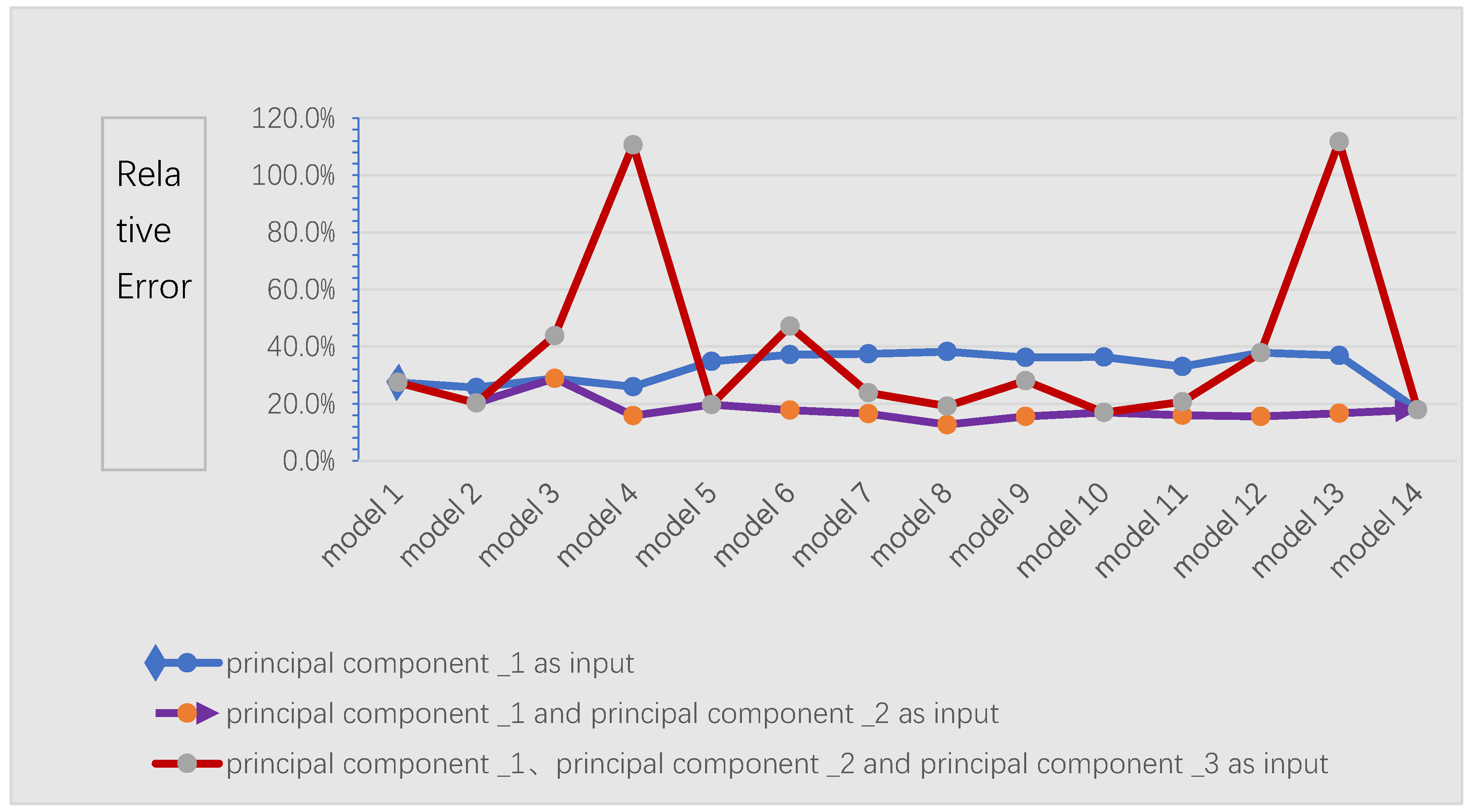
Figure 4 is plotted in order to compare the prediction effect of different network models with different principal component combinations as input. Figure 4 is the maximum relative error in Table 4, Table 5, and Table 6. As can be seen from Figure 4, with principal component _1 and principal component _2 as input of the Elman Neural Network, the performance of each model in the verification period is obviously better than that of principal component _1 or simultaneously with principal component _1, principal component _2 and principal component _3 as input of the Elman Neural Network.

3.2. Evaluation of Forecast Performance

According to the network structure determined by step 3.1.3, the Elman Neural Network model is trained by the average annual runoff data of Jinping hydropower station in 1960–2006 and tested by the average annual runoff data of Jinping hydropower station in 2007–2011.

The Mean Absolute Percentage Error (MAPE), Maximum Relative Error (MRE) and Qualified Rate (QR) are used as evaluation indexes for prediction. The indexes are calculated according to Equations (16) and (20)–(22). In the verification period, the error of the five forecasts is shown in

Table 7. Prediction error of single model in the verification period.

The Evaluation Index	Year	The First Time	The Second Time	The Third Time	The Fourth Time	The Fifth Time	Ensemble Forecast
RE	2007	14.10%	13.15%	11.41%	12.86%	15.24%	13.35%
	2008	−14.85%	−14.20%	−12.93%	−14.76%	−11.26%	−13.60%
	2009	1.63%	2.26%	3.70%	1.91%	6.57%	3.21%
	2010	4.63%	6.80%	7.97%	4.96%	6.78%	6.23%
	2011	−4.51%	−11.77%	−13.70%	−2.06%	−12.95%	−9.00%
QR		100%	100%	100%	100%	100%	100%
MRE		14.85%	14.20%	13.70%	14.76%	15.24%	13.60%
MAPE		7.94%	9.64%	9.94%	7.31%	10.56%	9.09%

. The predicted results are evaluated by mean absolute percent error, maximum relative error, and qualified rate.

In order to verify the generalization ability of the network model in this paper and the stability of the prediction, we carried out single model prediction 100 times. It is shown that the network model used in the invention has good generalization ability and prediction stability. The error statistics of the first five time forecasts are shown in Table 7.

As can be seen from Table 7, during the verification period, the maximum relative error of single forecast is within 16%, and the qualified rate is 100% according to the precision evaluation scheme of medium- and long-term runoff forecast [47]. This shows that the Elman Neural Network model driven by mutual information and KPCA has good generalization ability and predictive stability. The back propagation algorithm and momentum gradient updating algorithm are used to search the parameter space of the Elman Neural Network, and the error between the actual value of the historical runoff data and the predicted value of the Elman Neural Network is reduced through continuous training. However, the error surface may contain many different local minima, and in the search process of the parameter space of the Elman Neural Network, it may stay in the local minimum point, but not necessarily the global minimum point. Therefore, although the structure of each Elman Neural Network is the same, the parameters are different, which leads to the difference of the prediction results of each Elman Neural Network.

In order to reduce the deviation of prediction results caused by the uncertainty of model parameters, we carried out single model prediction of runoff several times; the average value of the results of multiple prediction is taken as the final prediction result. In this study, the average of 100 forecast results can be taken as the final forecast result.

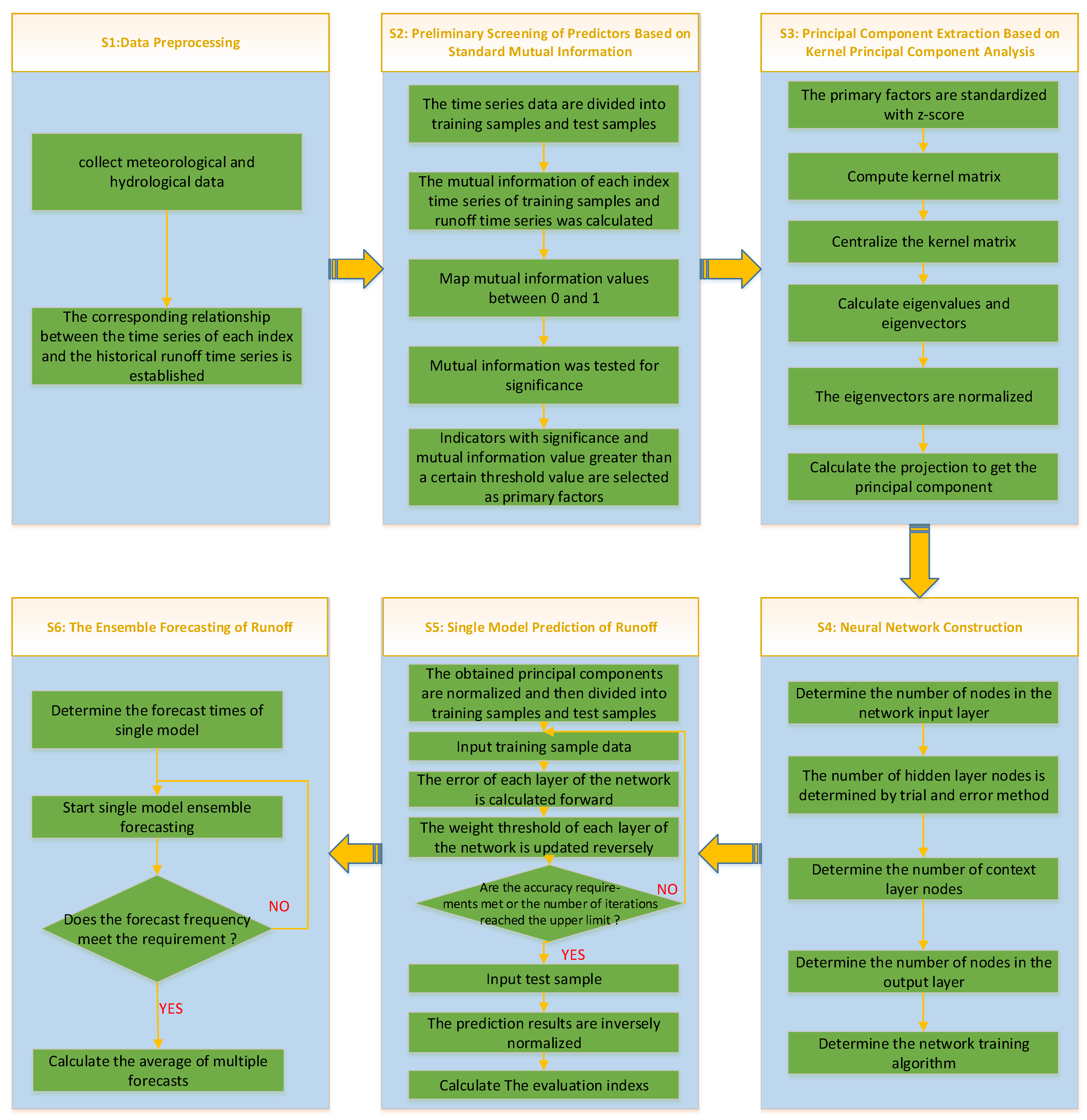
4. Conclusions

Due to the error of the original data and incompleteness of the model parameters, the prediction results between single prediction models may be quite different. This paper determined the prediction factors on the basis of rank correlation analysis, combined with the analysis of physical causes, and realized the single model forecast and multi-model set forecast of annual average runoff based on the Elman Neural Network, so as to provide reference for the medium- and long-term runoff forecast of reservoir. The general method flow described in this article is shown in Figure 5.

In detail, the automatic selection of predictors, the automatic feature extraction of predictors and the adaptive construction of the Elman Neural Network model are discussed, and the Elman Neural Network model driven by normalized mutual information and KPCA is proposed. This model is applied to the annual average runoff forecast of the Jinping I-Stage hydropower station in Sichuan, China, and the forecast results show that the factor screening method based on normalized mutual information and KPCA can effectively reduce noise and redundancy of a large number of predictors. Taking these factors as inputs, the Elman Neural Network has shown good generalization performance. High prediction stability, and prediction accuracy can meet actual production needs. The method of ensemble forecasting with multiple neural networks can effectively solve the problem of parameter uncertainty of the Elman Neural Network model and improve the accuracy of prediction. In addition, for a single prediction model based on the Elman neural network, prediction accuracy can meet the requirements but the prediction results between single prediction models may be quite different. Multi-model ensemble forecasting can reduce the influence of uncertainty and improve forecasting accuracy. However, due to error of the original data, the uncertainty of model parameters and environmental differences in different regions—and there are significant differences in modeling requirements for practical hydrological applications—more reliable and intelligent expert systems for real-time forecasting purposes need to be developed [48]. The multi-model ensemble prediction offers prediction deviation. How to determine the optimal ensemble prediction model needs to be further studied.

References

- Yaseen, Z.M.; El-Shafie, A.; Jaafar, O.; Afan, H.A.; Sayl, M.N. Artificial intelligence based models for stream-flow forecasting: 2000–2015. J. Hydrol. 2015, 530, 829–844. [Google Scholar] [CrossRef]
- Duan, Q.Y.; Sorooshian, S.; Gupta, V. Effective and efficient global optimization for conceptual Rainfall-runoff models. Water Resour. Res. 1992, 28, 1015–1031. [Google Scholar] [CrossRef]
- Kneis, D.; Burger, G.; Bronstert, A. Evaluation of medium-range runoff forecasts for a 500 km2 watershed. J. Hydrol. 2012, 414, 341–353. [Google Scholar] [CrossRef]
- Wang, W.C.; Chau, K.W.; Xu, D.M.; Chen, X.Y. Improving forecasting accuracy of annual runoff time series using ARIMA based on EEMD decomposition. Water Resour. Manag. 2015, 29, 1–21. [Google Scholar] [CrossRef]
- Chau, K.W. Use of Meta-Heuristic Techniques in Rainfall-Runoff Modelling. Water 2017, 9, 186. [Google Scholar] [CrossRef]
- Wang, W.; Ma, J. Review on some methods for hydrological forecasting. Adv. Sci. Technol. Water Res. 2005, 5, 6–60. [Google Scholar]
- Kisi, O.; Nia, A.M.; Goshen, M.G.; Tajabadi, M.R.J.; Ahmadi, A. Intermittent streamflow forecasting by using several data driven techniques. Water Resour. Manag. 2012, 26, 457–474. [Google Scholar] [CrossRef]
- Ge, Z.X.; Xue, M.; Song, Y.L. Application of multi-factor stepwise regression cycle analysis in medium and long-term hydrological forecast. J. HHU 2009, 37, 255–257. [Google Scholar]
- YAO, L.S.; CAI, Y.D. Long-range runoff forecast by artificial neural network. Adv. Water Sci. 1995, 6, 61–65. [Google Scholar]
- Machado, F.; Mine, M.; Kaviski, E.; Fill, H. Monthly rainfall-runoff modelling using artificial neural networks. Hydrol. Sci. J. 2011, 56, 349–361. [Google Scholar] [CrossRef]
- Alvaro, L.R.; Vicente, L.F.; David, P.V.; Joaquin, T.P. One-Day-Ahead Streamflow forecasting using artificial neural networks and a meteorological mesoscale model. J. Hydrol. Eng. 2015, 20. [Google Scholar] [CrossRef]
- Kisi, O.; Cimen, M. A wavelet-support vector machine conjunction model for monthly streamflow forecasting. J. Hydrol. 2011, 399, 132–140. [Google Scholar] [CrossRef]
- Huang, S.Z.; Chang, J.X.; Huang, Q.; Chen, Y.T. Monthly streamflow prediction using modified EMD-based support vector machine. J. Hydrol. 2014, 511, 764–775. [Google Scholar] [CrossRef]
- Liu, Z.Y.; Zhou, P.; Chen, G.; Guo, L.D. Evaluating a coupled discrete wavelet transform and support vector regression for daily and monthly streamflow forecasting. J. Hydrol. 2014, 519, 2822–2831. [Google Scholar] [CrossRef]
- Yang, L.; Tian, F.Q.; Hu, H.P. Modified ESP with information on the atmospheric circulation and teleconnection incorporated and its application. J. Tsinghua Univ. Sci. Tech. 2013, 53, 606–612. [Google Scholar]
- Day, G.N. Extended streamflow forecasting using NWSRFS. J. Water Resour. Manag. 1985, 111, 157–170. [Google Scholar] [CrossRef]
- Alan, F.; Dennis, H.; Lettenmaier, P. Columbia River streamflow forecasting based on ENSO and PDO climate signals. J. Water Resour. Plan. Manag. 1999, 125, 333–341. [Google Scholar]
- Lamb, K.; Piechota, T.; Moradkhani, H. Improving Ensemble Streamflow Prediction Using Interdecadal/Interannual Climate Variability; University of Nevada: Las Vegas, NV, USA, 2010. [Google Scholar]
- Werner, K.; Brandon, D.; Clark, M.; Gangopadhyay, S. Climate Index Weighting Schemes for NWS ESP-Based Seasonal Volume Forecasts. J. Hydrometeorol. 2004, 4, 1076–1090. [Google Scholar] [CrossRef]
- Gan, T.Y.; Gobena, A. Incorporation of seasonal climate forecasts in the ensemble streamflow prediction system. J. Hydrol. 2010, 385, 336–352. [Google Scholar]
- Druce, D.J. Insights from a history of seasonal inflow forecasting with a conceptual hydrologic model. J. Hydrol. 2001, 249, 102–112. [Google Scholar] [CrossRef]
- Kung, H.T.; Lin, L.Y.; Malasri, S. Use of Artificial Neural Networks in Precipitation Forecasting. In Regional Hydrological Response to Climate Change; Jones, J.A.A., Liu, C., Woo, M.K., Kung, H.T., Eds.; The GeoJournal Library; Springer: Dordrecht, The Netherlands, 1996; vol 38. [Google Scholar]
- Zhu, M.L.; Fujita, M.; Hashimoto, N. Application of Neural Networks to Runoff Prediction. In Stochastic and Statistical Methods in Hydrology and Environmental Engineering; Springer: Basel, Switzerland, 1993; pp. 205–216. [Google Scholar]
- Chen, S.; Wang, D. Genetic algorithms-based fuzzy optimization BP neural network model and its application. J. Hydraul. Eng. 2003, 5, 116–120. [Google Scholar]
- Standard for Hydrological Information and Hydrological Forecasting; GB/T 22482-2008; China Standard Press: Beijing, China, 2008; pp. 4–10.
- Sadeghi, B. A BP-neural network predictor model for plastic injection molding process. J. Mater. Process. Technol. 2000, 103, 411–416. [Google Scholar] [CrossRef]
- Shoaib, M.; Shamseldin, A.Y.; Melville, B.W.; Khan, M.M. A comparison between wavelet based static and dynamic neural network approaches for runoff prediction. J. Hydrol. 2016, 535, 211–225. [Google Scholar] [CrossRef]
- Guo, R.; Zhao, F.; Li, Y. Dynamic modeling of rainfall runoff process in river basin with recurrent wavelet neural network. J. Hydroelectr. Eng. 2013, 32, 55–59. [Google Scholar]
- Song, H.; Song, Y.; Zhang, D.; Zhong, W. Research on runoff forecasting of reservoir by using fuzzy clustering analysis and wavelet neural networks. J. Hydroelectr. Eng. 2008, 27, 6–10. [Google Scholar]
- Gao, X.; Zhang, J. Research on optimization of neural network based on genetic algorithm. Equip. Manuf. Technol. 2010, 2, 8–10. [Google Scholar]
- Shao, Y.; Lin, B.; Ye, J.; Liu, Y. Application of rainfall-runoff simulation based on Elman recurrent dynamic neural network model. J. Atmos. Sci. 2014, 37, 223–228. [Google Scholar]
- Zhang, X.; Shen, B.; Huang, L. Grey self-memory model based on BP neural network for annual runoff prediction. J. Hydroelectr. Eng. 2009, 28, 69–77. [Google Scholar]
- Jeffrey, L. Finding Structure in Time. Cogn. Sci. 1990, 14, 179–211. [Google Scholar]
- Chiang, Y.M.; Chang, L.C.; Chang, F.J. Comparison of static-feedforward and dynamic-feedback neural networks for rainfall-runoff modeling. J. Hydrol. 2004, 290, 297–311. [Google Scholar] [CrossRef]
- Wang, C.; Gao, X.; Xu, L.; Zhang, X. A new modified Elman neural network model. J. Electron. 1997, 19, 793. [Google Scholar]
- Gu, Y. Study on Monthly Runoff Forecasting Scheme of Hongjiadu Hydropower Station. Ph.D. Thesis, HoHai University, Nanjing, China, 2007. [Google Scholar]
- Feng, X.; Wang, Y.; Liu, Y.; Hu, Q. Monthly runoff forecast for Danjiangkou reservoir based on physical statistical methods. J. Hohai Univ. Nat. Sci. 2011, 39, 242–247. [Google Scholar]
- Slingo, J.; Palmer, T. Uncertainty in weather and climate prediction. Phil. Trans. R. Soc. A 2011, 369, 4751–4767. [Google Scholar] [CrossRef] [PubMed]
- Wang, Y.; Pan, H.; Ou, G.; Gong, Q.; Wei, X. Prediction of Debris Flow Runoff Process Based on Hydrological Model: A Case Study at Shenxi Gully, Regarding a Long-Term Impact by Wenchuan Earthquake. J. Donghua Univ. 2017, 34, 398–404. [Google Scholar]
- Zhao, T.; Yang, D. Prediction factor selection method based on mutual information in neural network runoff prediction model. J. Hydroelectr. Power 2011, 30, 24–30. [Google Scholar]
- Tang, H.; Wu, Y. Diagnosis of hydraulic cylinder leakage fault based on PCA and BP network. J. Cent. South Univ. 2011, 42, 3709–3714. [Google Scholar]
- Chen, Y.; Wang, W.S.; Tao, C.H.; Zhao, F. The Influence of climate change on runoff in the Yalong River Basin. Yangtze River 2012, 43, 25–29. [Google Scholar]
- Yu, W. Mutual Information and Clone Selection Algorithm Based Hyperspectral Band Selection Method. In Proceedings of the 36th China control conference, Dalian, China, 26–28 July 2017. [Google Scholar]
- Dan, L.; Xu, W.; Zheng, L.; Jiang, Y.; Xin, Z. Analysis on the changes of wetland in the lower reaches of weihe river in recent 16 years. Resour. Environ. Arid Areas 2019, 33, 112–118. [Google Scholar]
- Liu, Y.; Xin, W. Building facade image repeat texture detection method based on mutual information. Surv. Mapp. Geogr. Inf. 2018, 43, 93–95. [Google Scholar]
- Xie, X.; Tang, H.; Wang, J. Flood season runoff prediction model based on meteorological factors. Sci. Hydropower Energy 2015, 33, 10–12. [Google Scholar]
- David, E.; James, R.; McClelland, L. The PDP Research Group. Parallel Distributed Processing: Explorations in the Microstructure of Cognition; MIT Press: Cambridge, CA, USA, 1986; pp. 318–336. [Google Scholar]
- Yaseen, Z.M.; Sulaiman, S.O.; Deo, R.C.; Chau, K. An enhanced extreme learning machine model for river flow forecasting: State-of-the-art, practical applications in water resource engineering area and future research direction. J. Hydrol. 2018, 569, 387–408. [Google Scholar] [CrossRef]
Figure 1.
Location of the study area.
Figure 2.
Structure of the Elman Neural Network.
Figure 3.
Automatic iteration flow chart for runoff forecasting.
Figure 4.
Maximum relative error of each model in the verification period.
Figure 5.
General method flow chart.